When working with ML models such as GBMs, RFs, SVMs or kNNs (any one that is not a logistic regression) we can observe a pattern that is intriguing: the probabilities that the model outputs do not correspond to the real fraction of positives we see in real life. Can we solve this issue?

Motivated by sklearn’s topic Probability Calibration and the paper Practical Lessons from Predicting Clicks on Ads at Facebook, I’ll show how we can calibrate the output probabilities of a tree-based model while also improving its accuracy, by stacking it with a logistic regression.

Data

Let us use the credit card default dataset from UCI. The data is 30K rows long and 25 features wide, recording default payments, demographic factors, credit data, history of payment, and bill statements. The target variable is imbalanced, with the minority class representing 22% of records.

# reading the data
df = pd.read_csv('./UCI_Credit_Card.csv')

# let us check the data
df.head()

ID	LIMIT_BAL	SEX	EDUCATION	MARRIAGE	AGE	PAY_0	PAY_2	PAY_3	PAY_4	…	BILL_AMT4	BILL_AMT5	BILL_AMT6	PAY_AMT1	PAY_AMT2	PAY_AMT3	PAY_AMT4	PAY_AMT5	PAY_AMT6	default.payment.next.month
1	20000.0	2	2	1	24	2	2	-1	-1	…	0.0	0.0	0.0	0.0	689.0	0.0	0.0	0.0	0.0	1
2	120000.0	2	2	2	26	-1	2	0	0	…	3272.0	3455.0	3261.0	0.0	1000.0	1000.0	1000.0	0.0	2000.0	1
3	90000.0	2	2	2	34	0	0	0	0	…	14331.0	14948.0	15549.0	1518.0	1500.0	1000.0	1000.0	1000.0	5000.0	0
4	50000.0	2	2	1	37	0	0	0	0	…	28314.0	28959.0	29547.0	2000.0	2019.0	1200.0	1100.0	1069.0	1000.0	0
5	50000.0	1	2	1	57	-1	0	-1	0	…	20940.0	19146.0	19131.0	2000.0	36681.0	10000.0	9000.0	689.0	679.0	0

Cool. The data is tidy with only numeric columns. Let us move to modeling.

Modeling

Let us build up our calibrated models in steps. First, we set up the problem and run a vanilla Gradient Boosting Machine and a vanilla Extremely Randomized Trees model.

# getting design matrix and target
X = df.copy().drop(['ID','default.payment.next.month'], axis=1)
y = df.copy()['default.payment.next.month']

# defining the validation process
skf = StratifiedKFold(n_splits=5, shuffle=True, random_state=101)

Vanilla Gradient Boosting Machine

Let us get validation predictions from a lightgbm model.

# parameters obtained via random search
params = {'boosting_type': 'gbdt',
          'n_estimators': 100,
          'learning_rate': 0.012506,
          'class_weight': None,
          'min_child_samples': 51,
          'subsample': 0.509384,
          'colsample_bytree': 0.711932,
          'num_leaves': 76}

# configuring the model
lgbm = LGBMClassifier(**params)

# running CV
preds = cross_val_predict(lgbm, X, y, cv=skf, method='predict_proba')

# evaluating
roc_auc_score(y, preds[:,1])

0.784120

Our model shows an AUC of 0.784, which is a nice result in comparison to some experiments published by Kaggle users. Let us now check the probability calibration.

# creating a dataframe of target and probabilities
prob_df_lgbm = pd.DataFrame({'y':y, 'y_hat': preds[:,1]})

# binning the dataframe, so we can see success rates for bins of probability
bins = np.arange(0.05, 1.00, 0.05)
prob_df_lgbm.loc[:,'prob_bin'] = np.digitize(prob_df_lgbm['y_hat'], bins)
prob_df_lgbm.loc[:,'prob_bin_val'] = prob_df_lgbm['prob_bin'].replace(dict(zip(range(len(bins)), bins)))

# opening figure
plt.figure(figsize=(12,7), dpi=150)

# plotting ideal line
plt.plot([0,1],[0,1], 'k--', label='ideal')

# plotting calibration for lgbm
calibration_y = prob_df_lgbm.groupby('prob_bin_val')['y'].mean()
calibration_x = prob_df_lgbm.groupby('prob_bin_val')['y_hat'].mean()
plt.plot(calibration_x, calibration_y, marker='o', label='lgbm')

# legend and titles
plt.title('Calibration plot for LGBM')
plt.xlabel('Predicted probability')
plt.ylabel('Actual fraction of positives')
plt.legend()

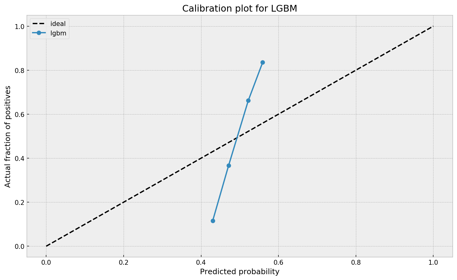
The calibration plot seems off. The model outputs a narrow interval of probabilities where it both overestimates and underestimates the true probability, depending on its output value. Let us now check how a Extremely Randomized Trees model performs.

Vanilla Extremely Randomized Trees

Let us try now the ExtraTreesClassifier from sklearn. We first search get model validation predictions:

# parameters obtained via random search
params = {'n_estimators': 100,
          'class_weight': 'balanced_subsample',
          'min_samples_leaf': 49,
          'max_features': 0.900676,
          'bootstrap': True,
          'n_jobs':-1}

# configuring the model
et = ExtraTreesClassifier(**params)

# running CV
preds = cross_val_predict(et, X, y, cv=skf, method='predict_proba')

# evaluating
roc_auc_score(y, preds[:,1]) 

0.784180

Cool. Our ET model also shows nice results, at AUC = 0.784, like the GBM model. We check the probability calibrations next.

# creating a dataframe of target and probabilities
prob_df_et = pd.DataFrame({'y':y, 'y_hat': preds[:,1]})

# binning the dataframe, so we can see success rates for bins of probability
bins = np.arange(0.05, 1.00, 0.05)
prob_df_et.loc[:,'prob_bin'] = np.digitize(prob_df_et['y_hat'], bins)
prob_df_et.loc[:,'prob_bin_val'] = prob_df_et['prob_bin'].replace(dict(zip(range(len(bins) + 1), list(bins) + [1.00])))

# opening figure
plt.figure(figsize=(12,7), dpi=150)

# plotting ideal line
plt.plot([0,1],[0,1], 'k--', label='ideal')

# plotting calibration for et
calibration_y = prob_df_et.groupby('prob_bin_val')['y'].mean()
calibration_x = prob_df_et.groupby('prob_bin_val')['y_hat'].mean()
plt.plot(calibration_x, calibration_y, marker='o', label='et')

# legend and titles
plt.title('Calibration plot for ET')
plt.xlabel('Predicted probability')
plt.ylabel('Actual fraction of positives')
plt.legend()

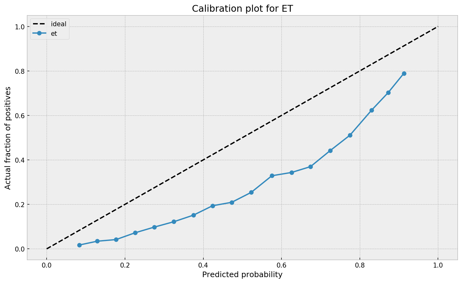
We can see that ETC overestimates the true probabilities across the board, despite having a wider probability range in comparison to GBM. Both models need a correction on their output probabilities. So how can we do that?

Logistic Regression on the leaves of forests

Let us show how to use a logistic regression on the leaves of forests in order to improve probability calibration. We first fit a tree-based model on the data, such as our lgbm:

# first, we fit our tree-based model on the dataset
lgbm.fit(X, y)

Then, we use the .apply method to get the indices of the leaves each sample ended up into.

# then, we apply the model to the data in order to get the leave indexes
leaves = lgbm.apply(X)
leaves

array([[ 11,  44,  50, ...,   1,   1,  27],
       [140,  69,  70, ...,  17, 125,  41],
       [149,  10, 219, ...,  90, 190, 154],
       ...,
       [164,  35, 205, ...,  56,  55, 168],
       [168,  50,  11, ..., 112, 188, 100],
       [119, 193, 216, ..., 197, 146, 201]])

We’re not yet ready to fit the logistic model on this matrix. So, we apply one-hot encoding to have dummies indicating leaf assignments:

# then, we one-hot encode the leave indexes so we can use them in the logistic regression
encoder = OneHotEncoder()
leaves_encoded = encoder.fit_transform(leaves)
leaves_encoded

<30000x22900 sparse matrix of type '<class 'numpy.float64'>'
	with 3000000 stored elements in Compressed Sparse Row format>

Now, we’re ready to fit the model. The leaves_encoded variable contains a very powerful feature transformation of the data, learned by the GBM model. For more info about this kind of transformation, refer to the Facebook paper I cited in the beginning of the post.

We configure the logistic regression so it has strong regularization (as the leaf encoding is high-dimensional) and no intercept. We also use the sag solver to speed things up.

# we configure the logistic regression and fit it to the encoded leaves
lr = LogisticRegression(solver='sag', C=10**(-3), fit_intercept=False)
lr.fit(leaves_encoded, y)

We can now compare the probabilities before and after the application of the logistic regression model. As it tries to minimize log-loss, we expect that its output probabilities are better calibrated. The scatterplot below shows the differences in probability calibration:

# let us check probabilities before and after logistic regression
preds_lgbmlr = lr.predict_proba(leaves_encoded)
preds_lgbm = lgbm.predict_proba(X)

# plotting the probabilities
plt.figure(figsize=(12,7), dpi=150)
plt.scatter(preds_lgbm[:,1], preds_lgbmlr[:,1], s=1)
plt.xlim(-0.05,1.05); plt.ylim(-0.05,1.05)

# adding text
plt.title('Comparison LGBM probabilities before and after Logistic Regression')
plt.xlabel('Probabilities before Logistic Regression')
plt.ylabel('Probabilities after Logistic Regression');

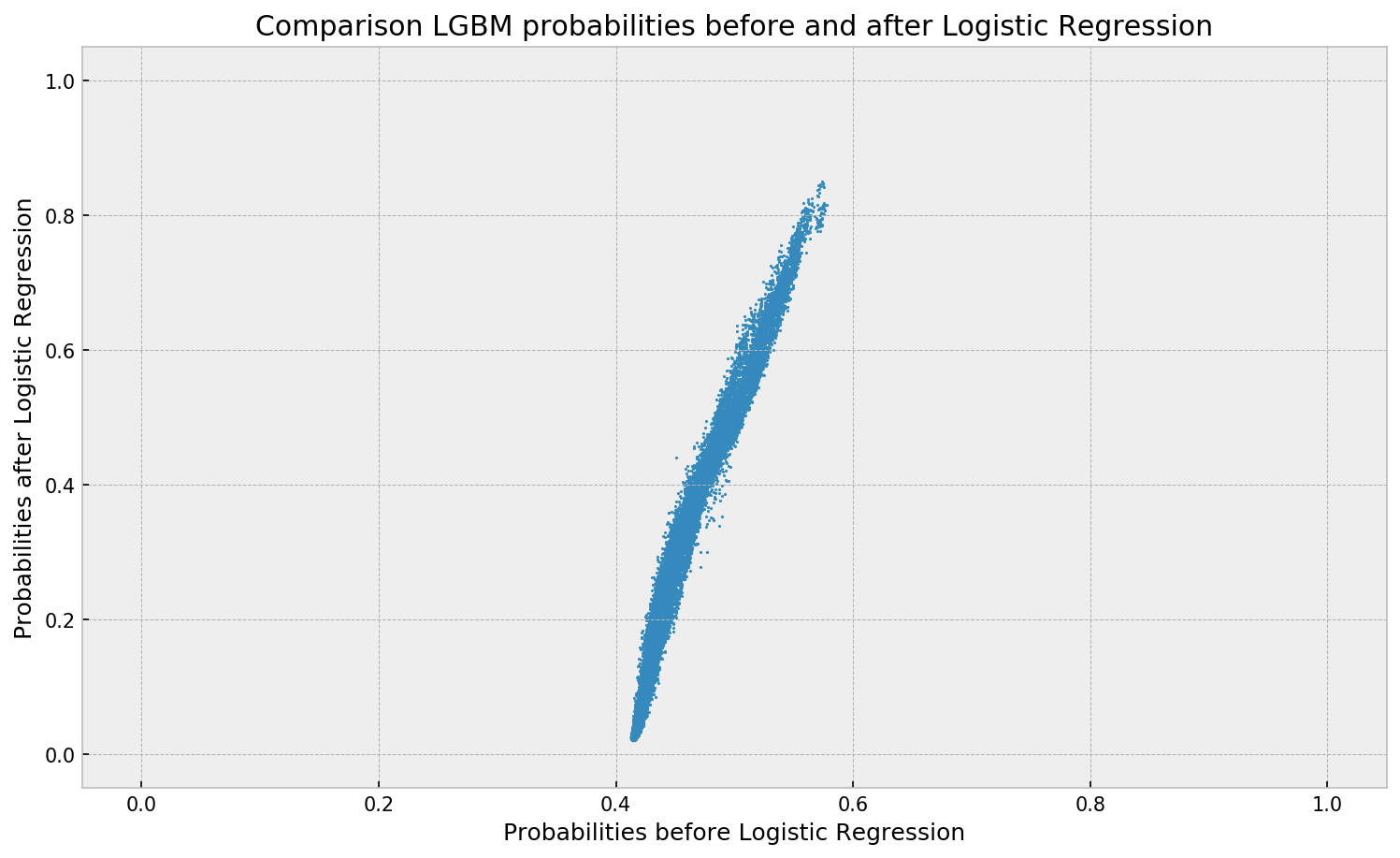
We can see the the range of the output probabilities is wider after the logistic regression. Also, the mapping resembles the calibration plot of LGBM, so LR may be actually correcting it.

However, we’re just analyzing training data. Let us build a robust pipeline so we can see the calibration plots in validation before taking any conclusions. The following class does just that:

# class for the tree-based/logistic regression pipeline
class TreeBasedLR:
    
    # initialization
    def __init__(self, forest_params, lr_params, forest_model):
        
        # storing parameters
        self.forest_params = forest_params
        self.lr_params = lr_params 
        self.forest_model = forest_model
        
    # method for fitting the model
    def fit(self, X, y, sample_weight=None):
        
        # dict for finding the models
        forest_model_dict = {'et': ExtraTreesClassifier, 'lgbm': LGBMClassifier}
        
        # configuring the models
        self.lr = LogisticRegression(**self.lr_params)
        self.forest = forest_model_dict[self.forest_model](**self.forest_params)
        self.classes_ = np.unique(y)
        
        # first, we fit our tree-based model on the dataset
        self.forest.fit(X, y)
        
        # then, we apply the model to the data in order to get the leave indexes
        leaves = self.forest.apply(X)
        
        # then, we one-hot encode the leave indexes so we can use them in the logistic regression
        self.encoder = OneHotEncoder()
        leaves_encoded = self.encoder.fit_transform(leaves)
        
        # and fit it to the encoded leaves
        self.lr.fit(leaves_encoded, y)
        
    # method for predicting probabilities
    def predict_proba(self, X):
        
        # then, we apply the model to the data in order to get the leave indexes
        leaves = self.forest.apply(X)
        
        # then, we one-hot encode the leave indexes so we can use them in the logistic regression
        leaves_encoded = self.encoder.transform(leaves)
        
        # and fit it to the encoded leaves
        y_hat = self.lr.predict_proba(leaves_encoded)
        
        # retuning probabilities
        return y_hat
    
    # get_params, needed for sklearn estimators
    def get_params(self, deep=True):
        return {'forest_params': self.forest_params,
                'lr_params': self.lr_params,
                'forest_model': self.forest_model}

We also change the seed of the validation so that the next model evaluations are fair:

# validation process
skf = StratifiedKFold(n_splits=5, shuffle=True, random_state=102)

Fixing LGBM probabilities

Let us calibrate the probabilities of our vanilla LGBM Model. The following code configures regularization paramter C of the logistic regression and fits it on the leaf assignments of our lgbm model. As stated earlier, we use a different random seed in the validation to get honest validation results.

# parameters obtained via random search
params = {'boosting_type': 'gbdt',
          'n_estimators': 100,
          'learning_rate': 0.012506,
          'class_weight': None,
          'min_child_samples': 51,
          'subsample': 0.509384,
          'colsample_bytree': 0.711932,
          'num_leaves': 76}
          
# parameters obtained via random search
lr_params = {'solver':'sag',
             'C': 0.001354,
             'fit_intercept': False}
             
# configuring the model
tblr = TreeBasedLR(tree_params, lr_params, forest_model='lgbm')

# running CV
preds = cross_val_predict(tblr, X, y, cv=skf, method='predict_proba')

# evaluating
roc_auc_score(y, preds[:,1])

0.783226

We approximately maintain original GBM results, with AUC = 0.783. Let us now check the calibration of this model:

# creating a dataframe of target and probabilities
prob_df_lgbm_lr = pd.DataFrame({'y':y, 'y_hat': preds[:,1]})

# binning the dataframe, so we can see success rates for bins of probability
bins = np.arange(0.05, 1.00, 0.05)
prob_df_lgbm_lr.loc[:,'prob_bin'] = np.digitize(prob_df_lgbm_lr['y_hat'], bins)
prob_df_lgbm_lr.loc[:,'prob_bin_val'] = prob_df_lgbm_lr['prob_bin'].replace(dict(zip(range(len(bins) + 1), list(bins) + [1.00])))

# opening figure
plt.figure(figsize=(12,7), dpi=150)

# plotting ideal line
plt.plot([0,1],[0,1], 'k--', label='ideal')

# plotting calibration for lgbm
calibration_y = prob_df_lgbm.groupby('prob_bin_val')['y'].mean()
calibration_x = prob_df_lgbm.groupby('prob_bin_val')['y_hat'].mean()
plt.plot(calibration_x, calibration_y, marker='o', label='lgbm')

# plotting calibration for lgbm+lr
calibration_y = prob_df_lgbm_lr.groupby('prob_bin_val')['y'].mean()
calibration_x = prob_df_lgbm_lr.groupby('prob_bin_val')['y_hat'].mean()
plt.plot(calibration_x, calibration_y, marker='o', label='lgbm+lr')

# legend and titles
plt.title('Calibration plot for LGBM, corrected')
plt.xlabel('Predicted probability')
plt.ylabel('Actual fraction of positives')
plt.legend()

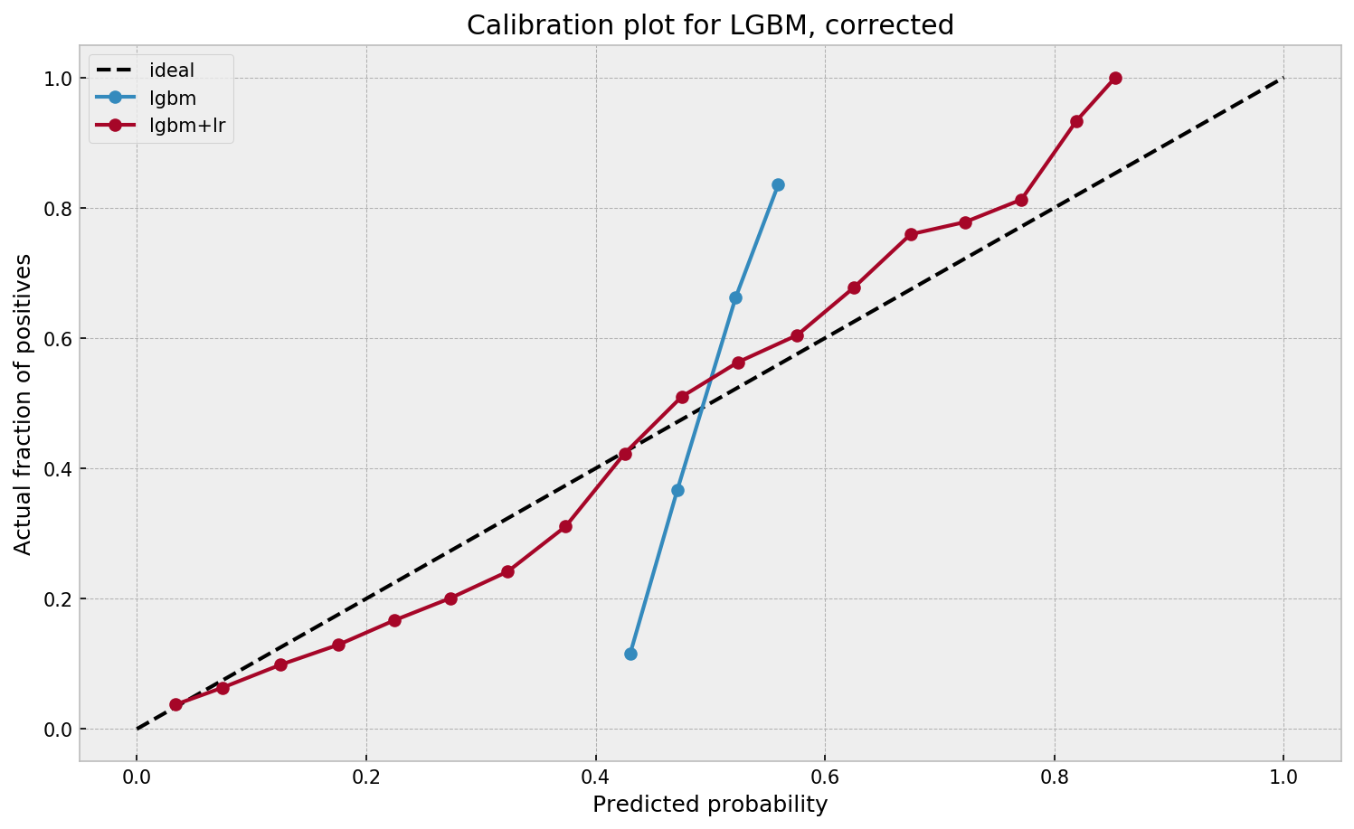
Much better. The calibration plot of lgbm+lr is much closer to the ideal. Now, when the model tells us that the probability of success is 60%, we can actually be much more confident that this is the true fraction of success! Let us now try this with the ET model.

Fixing ET probabilities

Same drill for our ExtraTreesClassifier:

# parameters obtained via random search
params = {'n_estimators': 100,
          'class_weight': 'balanced_subsample',
          'min_samples_leaf': 49,
          'max_features': 0.900676,
          'bootstrap': True,
          'n_jobs':-1}
          
# parameters obtained via random search
lr_params = {'solver':'sag',
             'C': 0.001756	,
             'fit_intercept': False}

# configuring the model
tblr = TreeBasedLR(tree_params, lr_params, forest_model='et')

# running CV
preds = cross_val_predict(tblr, X, y, cv=skf, method='predict_proba')

# evaluating
roc_auc_score(y, preds[:,1])

0.783781

No loss of AUC here as well, as the logistic model does a good job of learning from the forest’s leaves. Let us check the calibration:

# creating a dataframe of target and probabilities
prob_df_et_lr = pd.DataFrame({'y':y, 'y_hat': preds[:,1]})

# binning the dataframe, so we can see success rates for bins of probability
bins = np.arange(0.05, 1.00, 0.05)
prob_df_et_lr.loc[:,'prob_bin'] = np.digitize(prob_df_et_lr['y_hat'], bins)
prob_df_et_lr.loc[:,'prob_bin_val'] = prob_df_et_lr['prob_bin'].replace(dict(zip(range(len(bins) + 1), list(bins) + [1.00])))

# opening figure
plt.figure(figsize=(12,7), dpi=150)

# plotting ideal line
plt.plot([0,1],[0,1], 'k--', label='ideal')

# plotting calibration for et
calibration_y = prob_df_et.groupby('prob_bin_val')['y'].mean()
calibration_x = prob_df_et.groupby('prob_bin_val')['y_hat'].mean()
plt.plot(calibration_x, calibration_y, marker='o', label='et')

# plotting calibration for lgbm+lr
calibration_y = prob_df_et_lr.groupby('prob_bin_val')['y'].mean()
calibration_x = prob_df_et_lr.groupby('prob_bin_val')['y_hat'].mean()
plt.plot(calibration_x, calibration_y, marker='o', label='et+lr')

# legend and titles
plt.title('Calibration plot for ET, corrected')
plt.xlabel('Predicted probability')
plt.ylabel('Actual fraction of positives')
plt.legend()

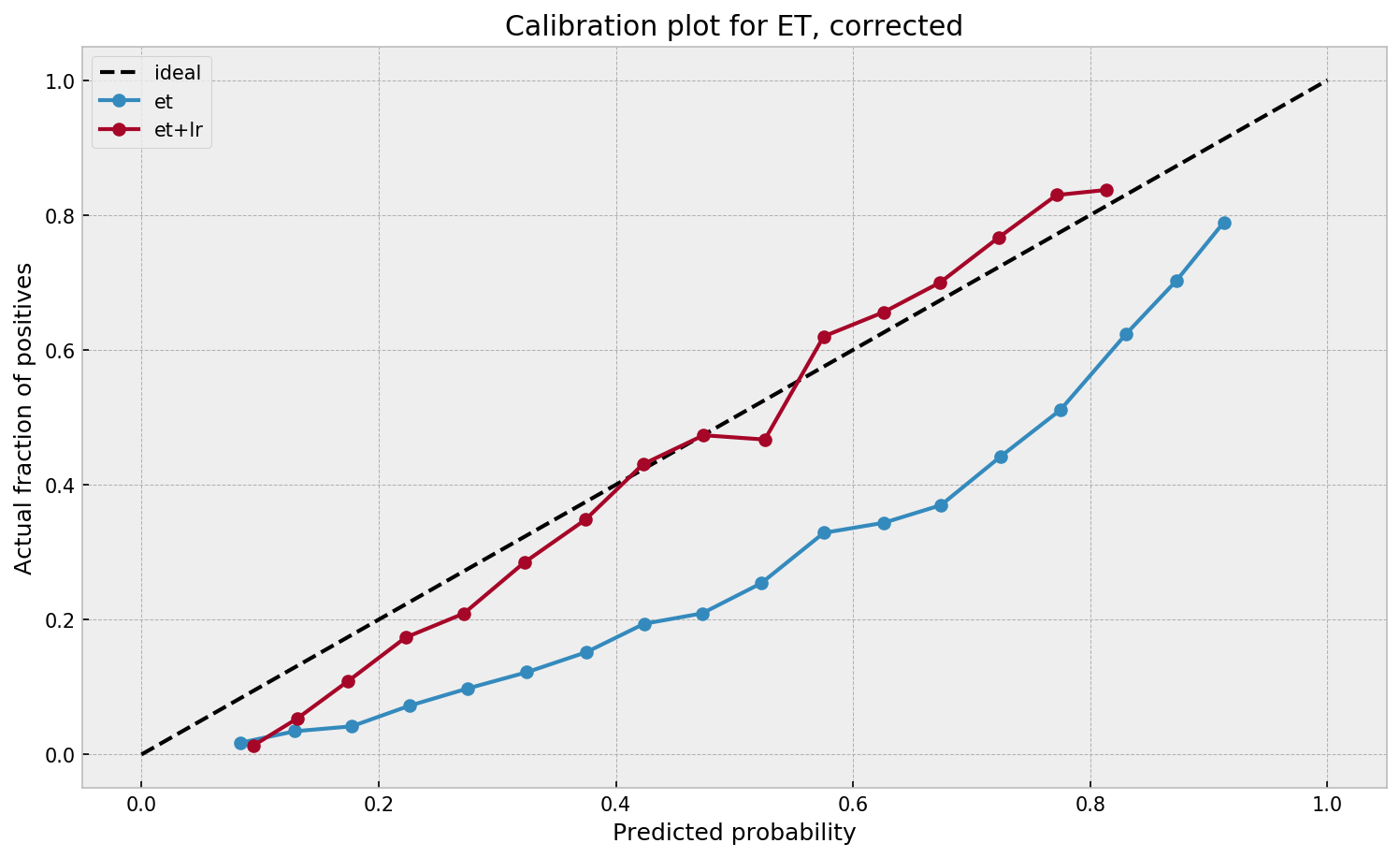
Calibration improves significantly as well. The process works for both models!

Conclusion

In this post, we showed a strategy to calibrate the output probabilities of a tree-based model by fitting a logistic regression on its one-hot encoded leaf assigments. The strategy greatly improves calibration while not losing predictive power. Thus, we can now be much more confident that the output probabilities of our models actually correspond to true fractions of success.

As always, you can find the complete code at my GitHub.