Thompson Sampling is a very simple yet effective method to addressing the exploration-exploitation dilemma in reinforcement/online learning. In this series of posts, I’ll introduce some applications of Thompson Sampling in simple examples, trying to show some cool visuals along the way. All the code can be found on my GitHub page here.

In this post, we explore the simplest setting of online learning: the Bernoulli bandit.

Problem: The Bernoulli Bandit

The Multi-Armed Bandit problem is the simplest setting of reinforcement learning. Suppose that a gambler faces a row of slot machines (bandits) on a casino. Each one of the $K$ machines has a probability $\theta_k$ of providing a reward to the player. Thus, the player has to decide which machines to play, how many times to play each machine and in which order to play them, in order to maximize his long-term cumulative reward.

At each round, we receive a binary reward, taken from an Bernoulli experiment with parameter $\theta_k$. Thus, at each round, each bandit behaves like a random variable $Y_k \sim \textrm{Bernoulli}(\theta_k)$. This version of the Multi-Armed Bandit is also called the Binomial bandit.

We can easily define in Python a set of bandits with known reward probabilities and implement methods for drawing rewards from them. We also compute the regret, which is the difference $\theta_{best} - \theta_i$ of the expected reward $\theta_i$ of our chosen bandit $i$ and the largest expected reward $\theta_{best}$.

# class for our row of bandits
class MAB:
    
    # initialization
    def __init__(self, bandit_probs):
        
        # storing bandit probs
        self.bandit_probs = bandit_probs
        
    # function that helps us draw from the bandits
    def draw(self, k):

        # we return the reward and the regret of the action
        return np.random.binomial(1, self.bandit_probs[k]), np.max(self.bandit_probs) - self.bandit_probs[k]

We can use matplotlib to generate a video of random draws from these bandits. Each row shows us the history of draws for the corresponding bandit, along with its true expected reward $\theta_k$. Hollow dots indicate that we pulled the arm but received no reward. Solid dots indicate that a reward was given by the bandit.

Cool! So how can we use this data in order to gather information efficiently and minimize our regret? Let us use tools from bayesian inference to help us with that!

Distributions over Expected Rewards

Now we start using bayesian inference to get a measure of expected reward and uncertainty for each of our bandits. First, we need a prior distribution, i.e., a distribution for our expected rewards (the $\theta_k$’s of the bandits). As each of our $K$ bandits is a bernoulli random variable with sucess probability $\theta_k$, our prior distribution over $\theta_k$ comes naturally (through conjungacy properties): the Beta distribution!

The Beta distribution, $\textrm{Beta}(1+\alpha, 1+\beta)$, models the parameter of a bernoulli random variable after we’ve observed $\alpha$ sucesses and $\beta$ failures. Let’s view some examples!

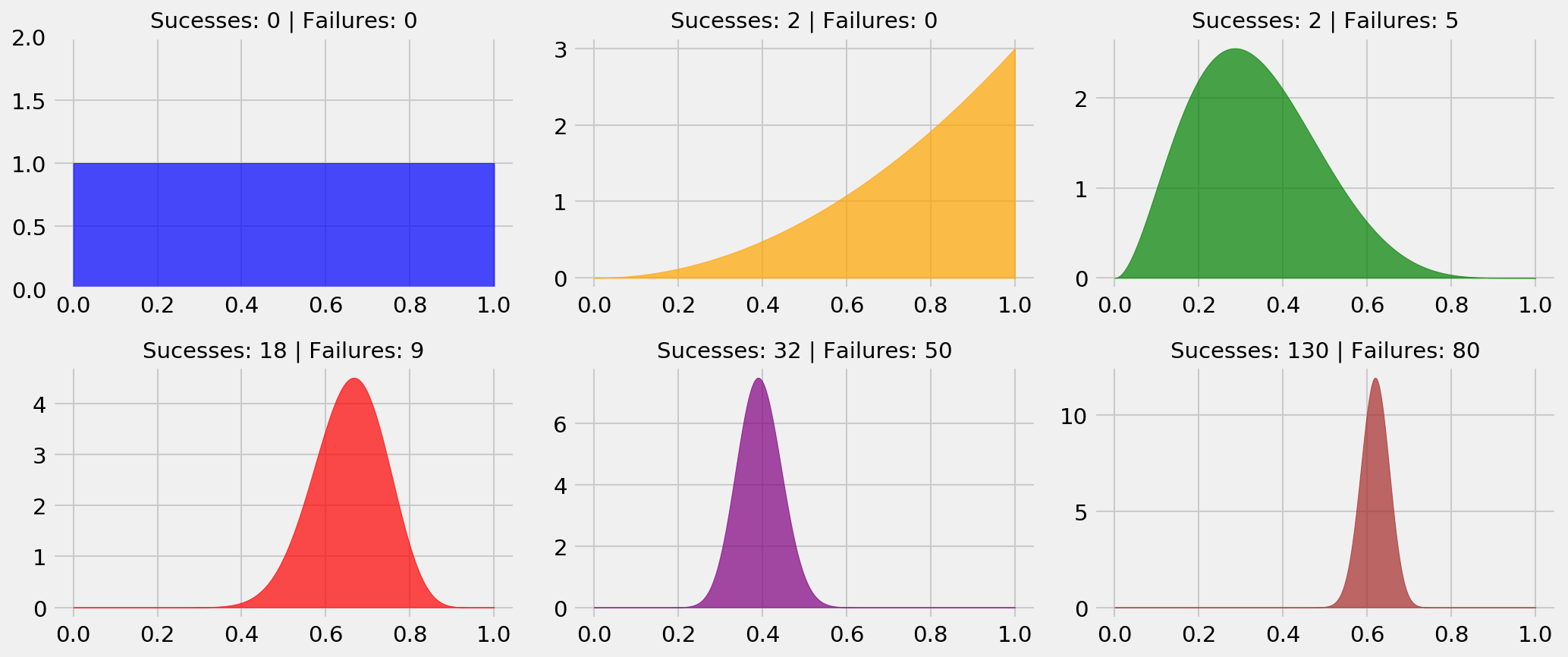
The interpretation is simple. In the blue plot, we haven’t started playing, so the only thing we can say about the probability of a reward from the bandit is that it is uniform between 0 or 1. This is our initial guess for $\theta_k$, our prior distribution. In the orange plot, we played two times and received two rewards, so we start moving probability mass to the right side of the plot, as we have evidence that the probability of getting a reward may be high. The distribution we get after updating our prior is the posterior distribution. In the green plot, we’ve played seven times and got two rewards, so our guess for $\theta_k$ is more biased towards the left-hand side.

As we play and gather evidence, our posterior distribution becomes more concentrated, as shown in the red, purple and brown plots. In the MAB setting, we calculate a posterior distribution for each bandit, at each round. The following video illustrates these updates.

The animation shows how the estimated probabilitites change as we play. Now, we can use this information to our benefit, in order to balance the uncertainty around our beliefs (exploration) with our objective of maximizing the cumulative reward (exploitation).

The Exploitation/Exploration Tradeoff

Now that we know how to estimate the posterior distribution of expected rewards for our bandits, we need to devise a method that can learn which machine to exploit as fast as possible. Thus, we need to balance how many potentially sub-optimal plays we use to gain information about the system (exploration) with how many plays we use to profit from the bandit we think is best (exploitation).

If we “waste” too many plays in random bandits just to gain knowledge, we lose cumulative reward. If we bet every play in a bandit that looked promising too soon, we can be stuck in a sub-optimal strategy.

This is what Thompson Sampling and other policies are all about. Let us first study other two popular policies, so we can compare them with TS: $\epsilon$-greedy and Upper Confidence Bound.

Mixing Random and Greedy Actions: $\epsilon$-greedy

The $\epsilon$-greedy policy is the simplest one. At each round, we select the best greedy action, but with $\epsilon$ probability, we select a random action (excluding the best greedy action).

In our case, the best greedy action is to select the bandit with the largest empirical expected reward, which is the one with the highest sample expected value $\textrm{argmax }\mathbf{E}[\theta_k]$. The policy is easily implemented with Python:

# e-greedy policy
class eGreedyPolicy:
    
    # initializing
    def __init__(self, epsilon):
        
        # saving epsilon
        self.epsilon = epsilon
    
    # choice of bandit
    def choose_bandit(self, k_array, reward_array, n_bandits):
        
        # sucesses and total draws
        success_count = reward_array.sum(axis=1)
        total_count = k_array.sum(axis=1)
        
        # ratio of sucesses vs total
        success_ratio = success_count/total_count
        
        # choosing best greedy action or random depending with epsilon probability
        if np.random.random() < self.epsilon:
            
            # returning random action, excluding best
            return np.random.choice(np.delete(list(range(N_BANDITS)), np.argmax(success_ratio)))
        
        # else return best
        else:
            
            # returning best greedy action
            return np.argmax(success_ratio)    

Let us observe how the policy fares in our game:

The $\epsilon$-greedy policy is our first step in trying to solve the bandit problem. It comes with a few caveats:

• Addition of a hyperaparameter: we have to tune $\epsilon$ to make it work. In most cases this is not trivial.
• Exploration is constant and inefficient: intuition tells us that we should explore more in the beginning and exploit more as time passes. The $\epsilon$-greedy policy always explores at the same rate. In the long term, if $\epsilon$ is not reduced, we’ll keep losing a great deal of rewards, even if we get little benefit from exploration. Also, we allocate exploration effort equally, even if empirical expected rewards are very different across bandits.
• High risk of suboptimal decision: if $\epsilon$ is low, we do not explore much, being under a high risk of being stuck in a sub-optimal bandit for a long time.

Let us now try a solution which uses the uncertainty over our reward estimates: the Upper Confidence Bound policy.

Optimism in the Face of Uncertainty: UCB

With the Upper Confidence Bound (UCB) policy we start using the uncertainty in our $\theta_k$ estimates to our benefit. The algorithm is as follows (UCB1 algorithm as defined here):

• For each action $j$ record the average reward $\overline{x_j}$ and number of times we have tried it $n_j$. We write $n$ for the total number of rounds.
• Perform the action that maximises $\overline{x_j} + \sqrt{\frac{2\textrm{ln} n}{n_j}}$

The algorithm will pick the arm that has the maximum value at the upper confidence bound. It will balance exploration and exploitation since it will prefer less played arms which are promising. The implementation follows:

# e-greedy policy
class UCBPolicy:
    
    # initializing
    def __init__(self):
        
        # nothing to do here
        pass
    
    # choice of bandit
    def choose_bandit(self, k_array, reward_array, n_bandits):
        
        # sucesses and total draws
        success_count = reward_array.sum(axis=1)
        total_count = k_array.sum(axis=1)
        
        # ratio of sucesses vs total
        success_ratio = success_count/total_count
        
        # computing square root term
        sqrt_term = np.sqrt(2*np.log(np.sum(total_count))/total_count)
        
        # returning best greedy action
        return np.argmax(success_ratio + sqrt_term)    

Let us observe how this policy fares in our game:

We can note that exploration is fairly heavy in the beginning, with exploitation taking place further on. The algorithm quickly adapts when a bandit becomes less promising, switching to another bandit with higher optimistic estimate. Eventually, it will solve the bandit problem, as it’s regret is bounded.

Now, for the last contender: Thompson Sampling!

Probability matching: Thompson Sampling

The idea behind Thompson Sampling is the so-called probability matching. At each round, we want to pick a bandit with probability equal to the probability of it being the optimal choice. We emulate this behaviour in a very simple way:

• At each round, we calculate the posterior distribution of $\theta_k$, for each of the $K$ bandits.
• We draw a single sample of each of our $\theta_k$, and pick the one with the largest value.

This algorithm is fairly old and did not receive much attention before this publication from Chapelle and Li, which showed strong empirical evidence of its efficiency. Let us try it for ourselves!

Code:

# e-greedy policy
class TSPolicy:
    
    # initializing
    def __init__(self):
        
        # nothing to do here
        pass
    
    # choice of bandit
    def choose_bandit(self, k_array, reward_array, n_bandits):

        # list of samples, for each bandit
        samples_list = []
        
        # sucesses and failures
        success_count = reward_array.sum(axis=1)
        failure_count = k_array.sum(axis=1) - success_count
                    
        # drawing a sample from each bandit distribution
        samples_list = [np.random.beta(1 + success_count[bandit_id], 1 + failure_count[bandit_id]) for bandit_id in range(n_bandits)]
                                
        # returning bandit with best sample
        return np.argmax(samples_list)    

And one simulation:

We can see that Thompson Sampling performs efficient exploration, quickly ruling out less promising arms, but not quite greedily: less promising arms with high uncertainty are activated, as we do not have sufficient information to rule them out. However, when the distribution of the best arm stands out, with uncertainty considered, we get a lot more agressive on exploitation.

But let us not take conclusions from an illustrative example with only 200 rounds of play. Let us analyze cumulative rewards and regrets for each of our decision policies in many long-term simulations.

Regrets and cumulative rewards

We have observed small illustrative examples of our decision policies, which provided us with interesting insights on how they work. Now, we’re interested in measuring their behaviour in the long-term, after many rounds of play. Therefore, and also to make things fair and minimize the effect of randomness, we will perform many simulations, and average the results per round across all simulations.

Regret after 10000 rounds

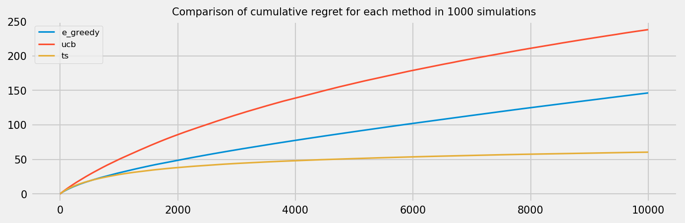
Let us inspect average regret on a game with 10k rounds for each policy. The plot below shows average results across 1000 simulations. We see that Thompson sampling greatly outperforms the other methods. It is noteworthy that the $\epsilon$-greedy strategy has linear cumulative regret, as it is always selecting random actions. An improvement could be the $\epsilon$-decreasing strategy, at a cost of more complexity to tune the algorithm. This may not be practical, as Thompson Sampling show better performance but has no hyperparameters. The UCB policy, in our experiment, shows worse results than the $\epsilon$-greedy strategy. We could improve the policy by using the UCB2 algorithm instead of UCB1, or by using a hyperparameter to control how optimistic we are. Nevertheless, we expect that UCB will catch up to $\epsilon$-greedy after more rounds, as it will stop exploring eventually.

Arm selection over time

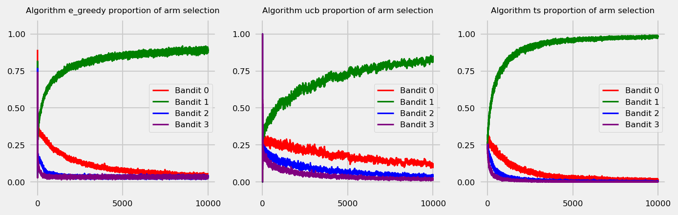
Let us take a look at the rates of arm selection over time. The plot below shows arm selection rates for each round averaged across 1000 simulations. Thompson Sampling shows quick convergence to the optimal bandit, and also more stability across simulations.

Conclusion

In this post, we showcased the Multi-Armed Bandit problem and tested three policies to address the exploration/exploitation problem: (a) $\epsilon$-greedy, (b) UCB and (c) Thompson Sampling.

The $\epsilon$-greedy strategy makes use of a hyperparameter to balance exploration and exploitation. This is not ideal, as it may be hard to tune. Also, the exploration is not efficient, as we explore bandits equally (in average), not considering how promising they may be.

The UCB strategy, unlike the $\epsilon$-greedy, uses the uncertainty of the posterior distribution to select the appropriate bandit at each round. It supposes that a bandit can be as good as it’s posterior distribution upper confidence bound. So we favor exploration by sampling from the distributions with high uncertainty and high tails, and exploit by sampling from the distribution with highest mean after we ruled out all the other upper confidence bounds.

Finally, Thompson Sampling uses a very elegant principle: to choose an action according to the probability of it being optimal. In practice, this makes for a very simple algorithm. We take one sample from each posterior, and choose the one with the highest value. Despite its simplicity, Thompson Sampling achieves state-of-the-art results, greatly outperforming the other algorithms. The logic is that it promotes efficient exploration: it explores more bandits that are promising, and quickly discards bad actions.