In earlier posts we explored the problem of estimating counterfactual outcomes, one of the central problems in causal inference, and learned that, with a few tweaks, simple decision trees can be a great tool for solving it. In this post, I’ll walk you thorugh the usage of DecisionTreeCounterfactual, one of the main models on the cfml_tools module, and see that it perfectly solves the toy causal inference problem from the fklearn library. You can find the full code for this example here.

Data: make_confounded_data from fklearn

Nubank’s fklearn module provides a nice causal inference problem generator, so we’re going to use the same data generating process and example from its documentation.

# getting confounded data from fklearn
from fklearn.data.datasets import make_confounded_data
df_rnd, df_obs, df_cf = make_confounded_data(50000)
print(df_to_markdown(df_obs.head(5)))

sex	age	severity	medication	recovery
0	34	0.7	1	126
1	24	0.72	1	123
1	38	0.86	1	255
1	35	0.77	1	227
0	22	0.078	0	15

We have five features: sex, age, severity, medication and recovery. We want to estimate the impact of medication on recovery. So, our target variable is recovery, our treatment variable is medication and the rest are our explanatory variables.

A good counterfactual model will tell us how would the recovery time be for each individual for both decisions of taking or not taking medication. The model should be robust to confounders, variables that impact the probability of someone taking the medication, or the effect of taking the medication. For instance, people with higher severity may be more likely to take the medicine. If not properly taken into account, this confounder may lead us to conclude that the medication may make recovery worse: people that took the medication may have worst recovery times (but their condition was already more severe). In the fklearn’s documentation, the data generating process is shown in detail, highlighting the confounders in the data. The effect we’re looking for is $exp(-1) = 0.368$.

The make_confounded_data function outputs three data frames: df_rnd, where treatment assingment is random, df_obs, where treatment assingment is confounded and df_cf, which is the counterfactual dataframe, containing the counterfactual outcome for all the individuals.

Let us try to solve this problem using DecisionTreeCounterfactual!

How DecisionTreeCounterfactual works

In causal inference, we aim to answer what would happen if we made a different decision in the past. This is quite hard because we cannot make two decisions simultaneously, or go back in time and check what would happen if we did things differently. However, what we can do is observe what happened to people who are similar to ourselves and made different choices. We do this all the time using family members, work colleagues, and friends as references.

But what it means to be similar, and most importantly, can similarity be learned? The answer is YES! For instance, when we run a decision tree, more than solving a classification or a regression problem, we’re dividing our data into clusters of similar elements given what features most explain our target. Thus, a decision tree works like a researcher deciding which variables to control to get the best effect estimate!

DecisionTreeCounterfactual leverages this supervised clustering approach and checks how changes on the treatment variable reflect on changes on the target given clusters determined by the explanatory variables that most impact the target. If we do not have any unobserved variable, we can be confident that the treatment variable really caused changes on the target, since everything else will be controlled.

Let us solve fklearn’s causal inference problem so we can walk though the method.

Easy mode: solving df_rnd

We call solving df_rnd “easy mode” because there’s no confounding, making it easy to estimate counterfactuals without paying attention to it. Nevertheless, it provides a good sanity check for DecisionTreeCounterfactual.

We first organize data in X (explanatory variables), W (treatment variable) and y (target) format, needed to fit DecisionTreeCounterfactual.

# organizing data into X, W and y
X = df_rnd[['sex','age','severity']]
W = df_rnd['medication']
y = df_rnd['recovery']

We then import the class and instantiate it.

# importing cfml-tools
from cfml_tools import DecisionTreeCounterfactual
dtcf = DecisionTreeCounterfactual(save_explanatory=True)

I advise that you read the docstring to know about the parameters and make the tutorial easier to follow!

Before fitting and getting counterfactuals, a good sanity check is doing 5-fold CV, to test the generalization power of the underlying tree model:

# validating model using 5-fold CV
cv_scores = dtcf.get_cross_val_scores(X, y)
print(cv_scores)

[0.54723148 0.57086291 0.56644823 0.56601209 0.543017]

Here, we have R2 scores in the range of ~0.55, which seem reasonable. However, there’s actually no baseline here: you just need to be confident that the model can capture and generalize relationships between explanatory variables and the target variable. Nevertheless, here are some tips: If your CV metric is too high (R2 very close to 1.00, for instance), it may mean that the treatment variable has no effect on the outcomes, or its effect is “masked” by correlated proxies in the explanatory variables. If your CV metric is too low (e.g. R2 close to 0), it does not mean that the model isn’t useful: the outcome may be explained only by the treatment variable.

We proceed to fit the model using X, W and y.

# fitting data to our model
dtcf.fit(X, W, y)

Calling .fit() builds a decision tree, solving the regression problem from X to y. But we actually use the decision tree as a supervised clustering algorithm. Each leaf of the tree determines a cluster of similar elements given the explanatory variables that most impact the target. Thus, we can calculate counterfactuals at the cluster level, by comparing the outcome of its elements for different W. .fit() is done when we have a table with counterfactuals by the tree’s leaves:

# showing counterfactual training table
print(df_to_markdown(dtcf.leaf_counterfactual_df.reset_index().head(6)))

leaf	W	y	count
7	0	11	73
7	1	30	62
9	0	12	51
9	1	31	54
10	0	13	69
10	1	34	102

We then predict the counterfactuals for all our individuals. By calling .predict(), we get the dataframe in the counterfactuals variable, which stores predictions for both W = 0 and W = 1. The counterfactuals are obtained running the samples in the tree, checking which cluster they’ve been assigned to, and querying the leaf_counterfactual_df built at .fit() for the outcome given different values of W.

# let us predict counterfactuals for these guys
counterfactuals = dtcf.predict(X)
counterfactuals.head()

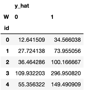
Then, we can compute treatment effects by using the counterfactual information:

# treatment effects
treatment_effects = counterfactuals['y_hat'][0]/counterfactuals['y_hat'][1]

And compare estimated effects vs real effects:

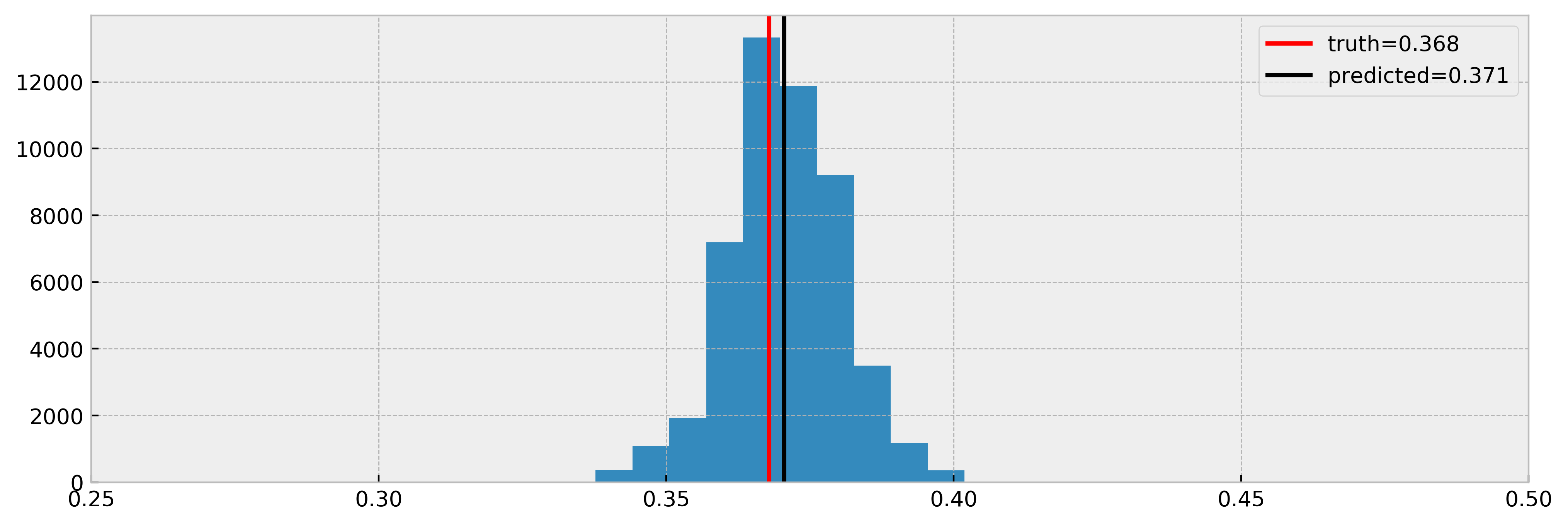
Cool! As we can see, the model nicely estimated the true effect.

This seems rather “black-boxy”. How can we trust the counterfactual predictions? We can use the DecisionTreeCounterfactual’s .explain() method! For a given test sample, it returns a table of comparable individuals with their treatment assignments and outcomes!

# our test sample
test_sample = X.iloc[[0]]
print(df_to_markdown(test_sample))

sex	age	severity
0	16	0.047

# running explanation
comparables_table = dtcf.explain(test_sample)

# showing comparables table
print(df_to_markdown(comparables_table.groupby('W').head(5).sort_values('W').reset_index()))

index	sex	age	severity	W	y
1444	0	15	0.049	0	13
2180	0	15	0.083	0	10
2379	0	15	0.045	0	13
3388	0	16	0.078	0	10
4036	0	15	0.056	0	18
0	0	16	0.047	1	31
71	0	16	0.089	1	35
157	0	14	0.07	1	30
1096	0	15	0.048	1	28
1412	0	14	0.093	1	34

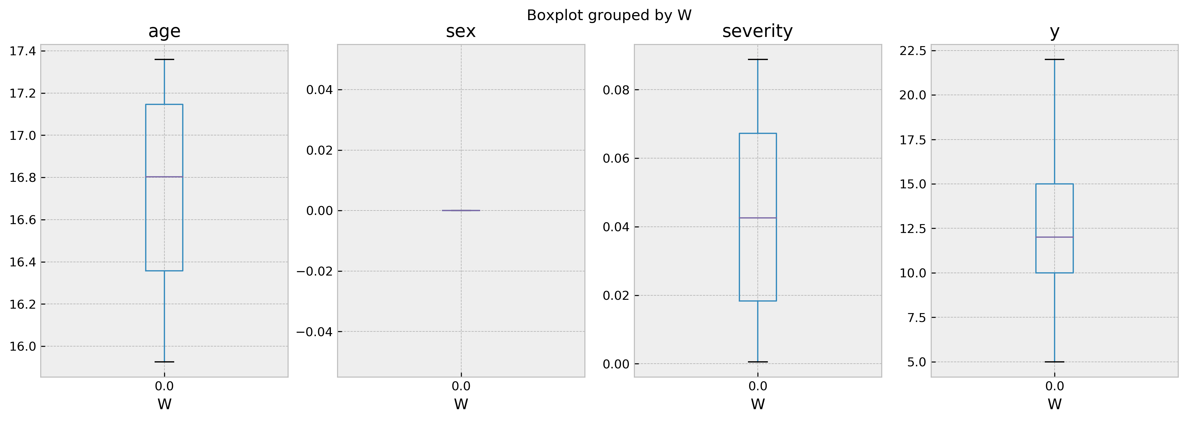
For a better visualization, you can check the following boxplot as well:

fig, ax = plt.subplots(1, 4, figsize=(16, 5), dpi=150)
comparables_table.boxplot('age','W', ax=ax[0])
comparables_table.boxplot('sex','W', ax=ax[1])
comparables_table.boxplot('severity','W', ax=ax[2])
comparables_table.boxplot('y','W', ax=ax[3])

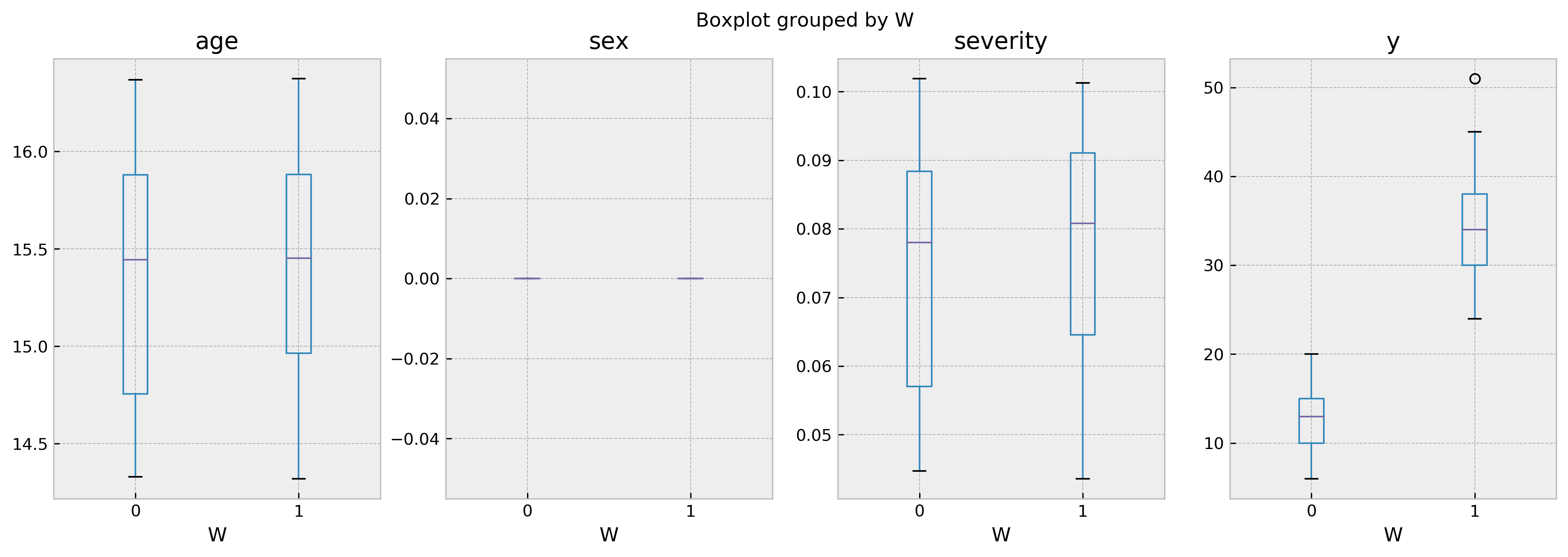
As the boxplot shows, both groups of treated and untreated individuals are very similar. Thus, we can be sure that the difference in the outcome is only due by the difference in the treatment. By looking at the results it becomes crystal clear that the treatment improves outcomes.

Let us now go for the “hard mode”, solving a counterfactual estimation problem with confounding.

Hard mode: solving df_obs

Now, we go for the “hard mode” and try to solve df_obs. Now we have confounding, which means that treatment assingment will not be uniform. Nevertheless, we run ForestEmbeddingsCounterfactual like before.

Organizing data in X, W and y format again:

# organizing data into X, W and y
X = df_obs[['sex','age','severity']]
W = df_obs['medication']
y = df_obs['recovery']

Validating the model, as before:

# importing cfml-tools
from cfml_tools import DecisionTreeCounterfactual
dtcf = DecisionTreeCounterfactual(save_explanatory=True)

# validating model using 5-fold CV
cv_scores = dtcf.get_cross_val_scores(X, y)
print(cv_scores)

[0.90593652 0.9394594 0.94191483 0.93571656 0.93803323]

Here it gets a little bit different. Remember that a high R2 could mean that the treatment variable has little effect on the outcome? As the treatment assignment is now correlated with the other variables, they “steal” importance from the treatment and this shows as a higher R2 in the confounded case.

We proceed to fit the model using X, W and y.

# fitting data to our model
dtcf.fit(X, W, y)

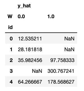
We then predict the counterfactuals for all our individuals. We get the dataframe in the counterfactuals variable, which predicts outcomes for both W = 0 and W = 1.

In this case, we can see some NaNs. That’s because for some individuals there are not enough treated or untreated neighbors to estimate the counterfactuals, controlled by the parameter min_sample_effect. When this parameter is high, we are conservative, getting more NaNs but less variance in counterfactual estimation.

# let us predict counterfactuals for these guys
counterfactuals = dtcf.predict(X)
counterfactuals.head()

Let us now compare true effect with estimated, for all the samples we could infer a counterfactual (no NaNs). Will the model get a good estimate in this case?

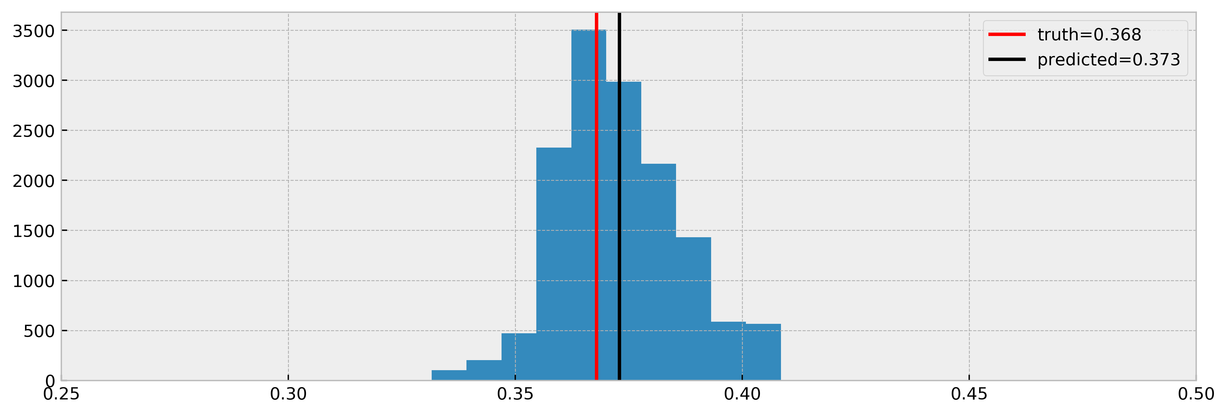
Nice! The model estimated the effect very well again. Note that we have less samples in the histogram, due to NaNs. Nevertheless, it is a cool result and shows that DecisionTreeCounterfactual can work with confounded data.

Let us explain the counterfactual of the first prediction, which is NaN for W = 1.

# our test sample
test_sample = X.iloc[[0]]

# running explanation
comparables_table = dtcf.explain(test_sample)

# showing comparables table
val_counts = comparables_table['W'].value_counts()
print(f'Number of treated: {val_counts[1]}, number of untreated: {val_counts[0]}')

Number of treated: 0, number of untreated: 142

In this case, there’s no treated comparables for us to draw inferences from. This explains why we cannot predict the outcome for this individual given W = 1! You can control the mininum number of samples required to perform a valid inference with the parameter min_sample_effect.

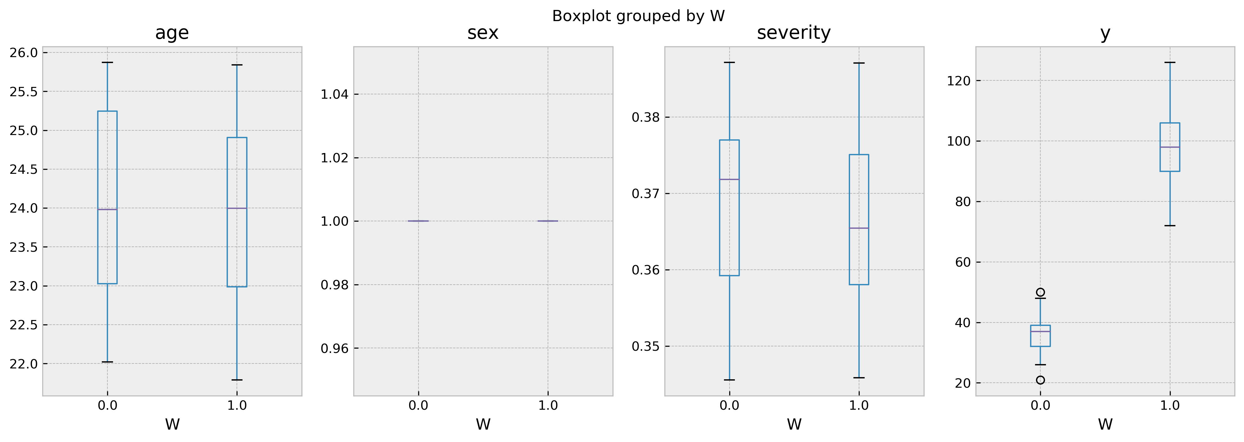
On the other hand, our third test sample has a healthy number of treated vs. untreated samples, so we can infer counterfactuals:

# our test sample
test_sample = X.iloc[[2]]

# running explanation
comparables_table = dtcf.explain(test_sample)

# showing comparables table
val_counts = comparables_table['W'].value_counts()
print(f'Number of treated: {val_counts[1]}, number of untreated: {val_counts[0]}')

Number of treated: 120, number of untreated: 57

I hope you liked the tutorial and will use cfml_tools for your causal inference problems soon!