In earlier posts we explored the problem of estimating counterfactual outcomes, one of the central problems in causal inference, and learned that, with a few tweaks, simple decision trees can be a great tool for solving it. In this post, I’ll walk you thorugh the usage of ForestEmbeddingsCounterfactual, one of the main models on the cfml_tools module, and see that it perfectly solves the toy causal inference problem from the fklearn library. You can find the full code for this example here.
Data: make_confounded_data from fklearn
Nubank’s fklearn module provides a nice causal inference problem generator, so we’re going to use the same data generating process and example from its documentation.
# getting confounded data from fklearn
from fklearn.data.datasets import make_confounded_data
df_rnd, df_obs, df_cf = make_confounded_data(50000)
print(df_to_markdown(df_obs.head(5)))
| sex | age | severity | medication | recovery |
|---|---|---|---|---|
| 0 | 34 | 0.7 | 1 | 126 |
| 1 | 24 | 0.72 | 1 | 123 |
| 1 | 38 | 0.86 | 1 | 255 |
| 1 | 35 | 0.77 | 1 | 227 |
| 0 | 22 | 0.078 | 0 | 15 |
We have five features: sex, age, severity, medication and recovery. We want to estimate the impact of medication on recovery. So, our target variable is recovery, our treatment variable is medication and the rest are our explanatory variables.
A good counterfactual model will tell us how would the recovery time be for each individual for both decisions of taking or not taking medication. The model should be robust to confounders, variables that impact the probability of someone taking the medication, or the effect of taking the medication. For instance, people with higher severity may be more likely to take the medicine. If not properly taken into account, this confounder may lead us to conclude that the medication may make recovery worse: people that took the medication may have worst recovery times (but their condition was already more severe). In the fklearn’s documentation, the data generating process is shown in detail, highlighting the confounders in the data. The effect we’re looking for is $exp(-1) = 0.368$.
The make_confounded_data function outputs three data frames: df_rnd, where treatment assingment is random, df_obs, where treatment assingment is confounded and df_cf, which is the counterfactual dataframe, containing the counterfactual outcome for all the individuals.
Let us try to solve this problem using ForestEmbeddingsCounterfactual!
How ForestEmbeddingsCounterfactual works
In causal inference, we aim to answer what would happen if we made a different decision in the past. This is quite hard because we cannot make two decisions simultaneously, or go back in time and check what would happen if we did things differently. However, what we can do is observe what happened to people who are similar to ourselves and made different choices. We do this all the time using family members, work colleagues, and friends as references.
But what it means to be similar, and most importantly, can similarity be learned? The answer is YES! For instance, when we run a decision tree, more than solving a classification or a regression problem, we’re dividing our data into clusters of similar elements given what features most explain our target. And if we repeat this process, such as building a Random Forest, we’ll note that some samples are more likely to end up together in the same leaf than others. Thus, we can measure similarity by counting at how many trees in the forest two elements ended up together in the same leaf!
ForestEmbeddingsCounterfactual leverages the embedding created by this leaf co-occurrence similarity metric to search for similar elements on the explanatory variables and check how changes on the treatment variable reflect on changes on the target. If we do not have any unobserved variable, we can be confident that the treatment variable really caused changes on the target, since everything else will be controlled.
Let us solve fklearn’s causal inference problem so we can walk through the method.
Easy mode: solving df_rnd
We call solving df_rnd “easy mode” because there’s no confounding, making it easy to estimate counterfactuals without paying attention to it. Nevertheless, it provides a good sanity check for ForestEmbeddingsCounterfactual.
We first organize data in X (explanatory variables), W (treatment variable) and y (target) format, needed to fit ForestEmbeddingsCounterfactual.
# organizing data into X, W and y
X = df_rnd[['sex','age','severity']]
W = df_rnd['medication']
y = df_rnd['recovery']
We then import the class and instantiate it.
# importing cfml-tools
from cfml_tools import ForestEmbeddingsCounterfactual
fecf = ForestEmbeddingsCounterfactual(save_explanatory=True)
I advise you to read the docstring to know about the parameters and make the tutorial easier to follow! Before fitting and getting counterfactuals, a good sanity check is doing 5-fold CV, to test the generalization power of the underlying forest model:
# validating model using 5-fold CV
cv_scores = fecf.get_cross_val_scores(X, y)
print(cv_scores)
[0.55879863 0.5832598 0.58331632 0.58258708 0.56651886]
Here, we have R2 scores in the range of ~0.55, which seem reasonable. However, there’s actually no baseline here: you just need to be confident that the model can capture and generalize relationships between explanatory variables and the target variable. Nevertheless, here are some tips: If your CV metric is too high (R2 very close to 1.00, for instance), it may mean that the treatment variable has no effect on the outcomes, or its effect is “masked” by correlated proxies in the explanatory variables. If your CV metric is too low (e.g. R2 close to 0), it does not mean that the model isn’t useful: the outcome may be explained only by the treatment variable. In this case, since the underlying model is a ExtraTreesRegressor the forest embedding would work as a unsupervised embedding, like sklearn’s RandomTreesEmbedding.
We proceed to fit the model using X, W and y.
# fitting data to our model
fecf.fit(X, W, y)
Calling .fit() builds the forest and creates a nearest neighbor index using leaf co-ocurrence as a similarity metric. For more details on that, check my earlier post about forest embeddings.
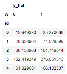
We then predict the counterfactuals for all our individuals. By calling .predict(), we get the dataframe in the counterfactuals variable, which stores predictions for both W = 0 and W = 1. The counterfactuals are obtained by querying the nearest neighbor index built on .fit() for n_neighbors and calculating the average outcome given different values of W.
# let us predict counterfactuals for these guys
counterfactuals = fecf.predict(X)
counterfactuals.head()
Then, we can compute treatment effects as follows:
# treatment effects
treatment_effects = counterfactuals['y_hat'][0]/counterfactuals['y_hat'][1]
And compare estimated effects vs real effects:
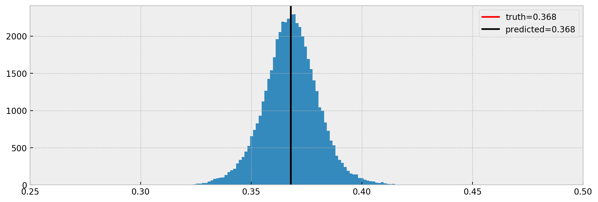
Cool! As we can see, the model nicely estimated the true effect.
But how can we be sure that the model is performing well? Let us do a quick diagnostic using a visualization of our forest embedding.
Diagnosis and criticism
A good diagnostic is to look at a 2D representation of our forest embedding, using UMAP:
# getting embedding from data
reduced_embed = fecf.get_umap_embedding(X)
Under the hood, UMAP takes our leaf-based similarity metric and creates a 2D representation that tries to preserve it. This shows natural clusters in our data, and surfaces what the model learned in terms of similarity and representation.
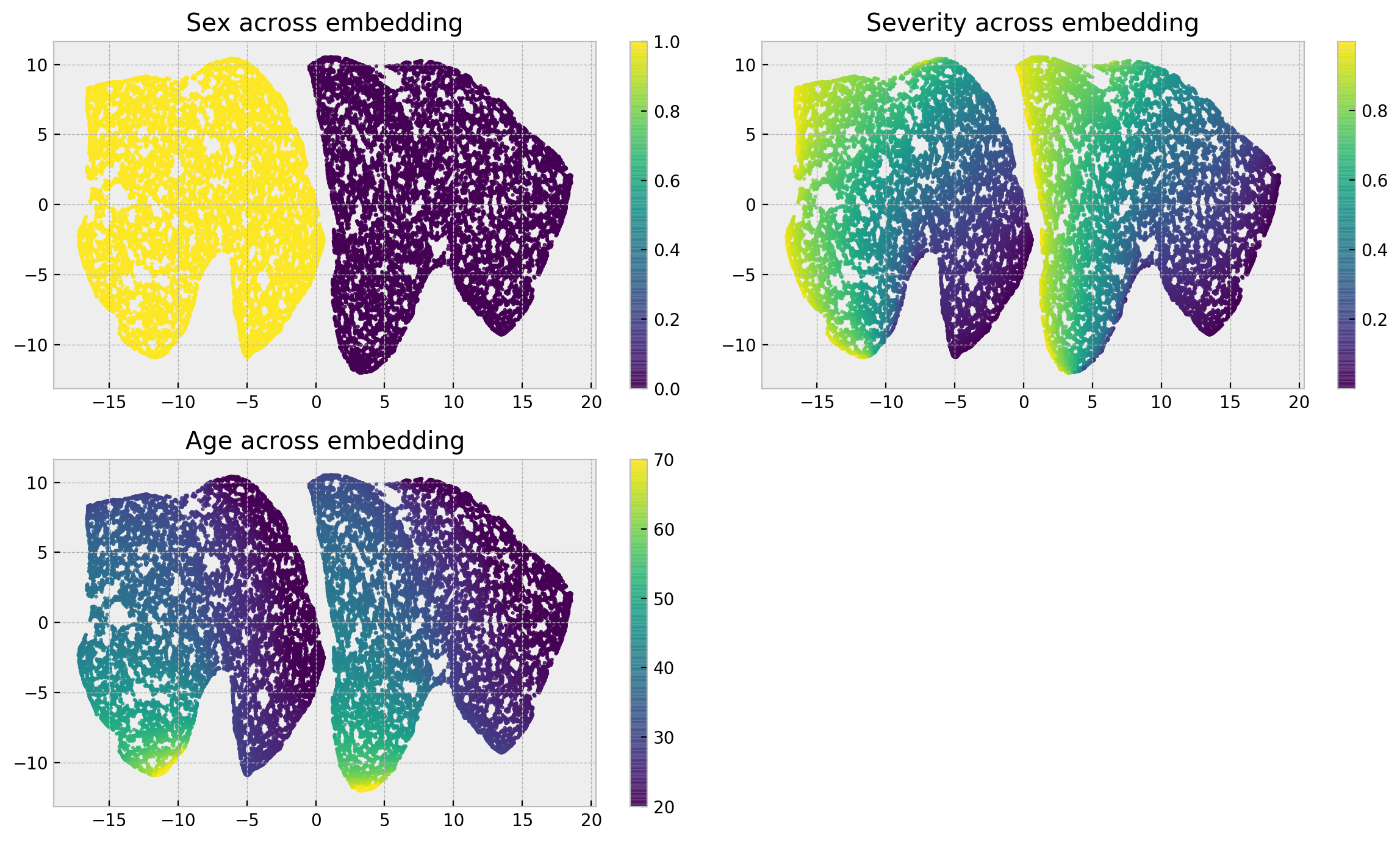
The plots show how our explanatory variables are distributed across the embedding. Sex breaks the embedding into two separate clusters, while severity is distributed in a left-right gradient inside each cluster and age follows an up-down gradient. The gradients are smooth enough such that we can be confident that at each local neighborhood individuals are very similar. Thus, the only thing that could explain differences in the outcomes of members of a local neighborhood is dispersion in the treatment variable!
Let us have a look at the outcomes and treatment assignments:
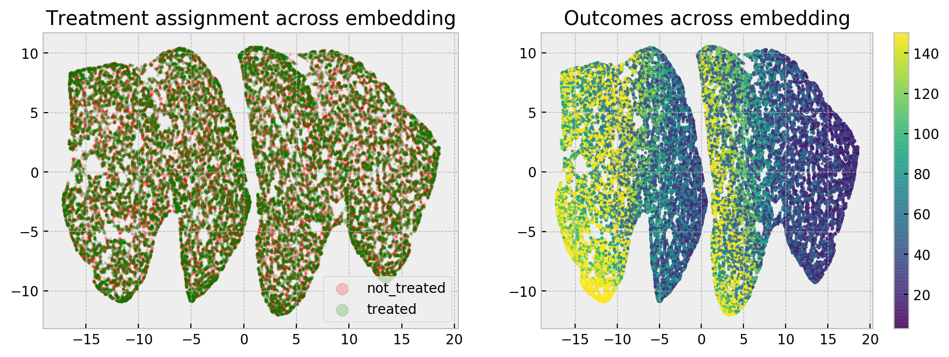
As we can see, treated and not treated individuals are uniformly scattered across the map, and the granular pattern in the right-hand side plot tells us that lack of treatment degrades outcomes for all local neighborhoods. That’s how we compute counterfactuals: comparing how the treatment variable impacts outcomes for similar individuals!
If you still need to dig deeper, ForestEmbeddingsCounterfactual implements a .explain() method so you can see which comparables the model used to calculate counterfactuals for a given sample.
# our test sample
test_sample = X.iloc[[0]]
print(df_to_markdown(test_sample))
| sex | age | severity |
|---|---|---|
| 0 | 16 | 0.047 |
# running explanation
comparables_table = fecf.explain(test_sample)

# showing comparables table
print(df_to_markdown(comparables_table.groupby('W').head(5).sort_values('W').reset_index()))
| index | sex | age | severity | W | y |
|---|---|---|---|---|---|
| 11594 | 0 | 16 | 0.048 | 0 | 18 |
| 990 | 0 | 16 | 0.048 | 0 | 15 |
| 35909 | 0 | 17 | 0.048 | 0 | 8 |
| 19406 | 0 | 16 | 0.039 | 0 | 10 |
| 23348 | 0 | 17 | 0.049 | 0 | 10 |
| 0 | 0 | 16 | 0.047 | 1 | 31 |
| 44725 | 0 | 16 | 0.049 | 1 | 39 |
| 43051 | 0 | 16 | 0.042 | 1 | 30 |
| 31859 | 0 | 17 | 0.046 | 1 | 43 |
| 28498 | 0 | 16 | 0.034 | 1 | 37 |
As you can see, the model found a lot of “twins” to the test sample with different treatment assignments and outcomes. By looking at the table it becomes crystal clear that the treatment improves outcomes.
Cool, right? The uniform assignment case is good to get the intuition about embeddings and usage of ForestEmbeddingsCounterfactual. Let us move to the case where treatment assignments are not uniformly distributed, making the counterfactual estimation harder (but still doable!).
Hard mode: solving df_obs
Now, we go for the “hard mode” and try to solve df_obs. Now we have confounding, which means that treatment assingment will not be uniform. Nevertheless, we run ForestEmbeddingsCounterfactual like before!
Organizing data in X, W and y format again:
# organizing data into X, W and y
X = df_obs[['sex','age','severity']]
W = df_obs['medication']
y = df_obs['recovery']
Validating the model, as before:
# importing cfml-tools
from cfml_tools import ForestEmbeddingsCounterfactual
fecf = ForestEmbeddingsCounterfactual(save_explanatory=True)

# validating model using 5-fold CV
cv_scores = fecf.get_cross_val_scores(X, y)
print(cv_scores)
[0.9543888 0.95643801 0.95538205 0.95339682 0.92864522]
Here it gets a little bit different. Remember that a high R2 could mean that the treatment variable has little effect on the outcome? As the treatment assignment is correlated with the other variables, they “steal” importance from the treatment and our R2 gets higher in the confounded case. This will become even clearer when we look at the UMAP embedding.
We proceed to fit the model using X, W and y.
# fitting data to our model
fecf.fit(X, W, y)
We then predict the counterfactuals for all our individuals.
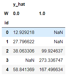
In this case, we can see some NaNs. That’s because some individuals do not have enough treated or untreated neighbors to estimate the counterfactuals, controlled by the parameter min_sample_effect. When this parameter is high, we are conservative, getting more NaNs but less variance in counterfactual estimation.
# let us predict counterfactuals for these guys
counterfactuals = fecf.predict(X)
counterfactuals.head()
Comparing true effect with estimated:
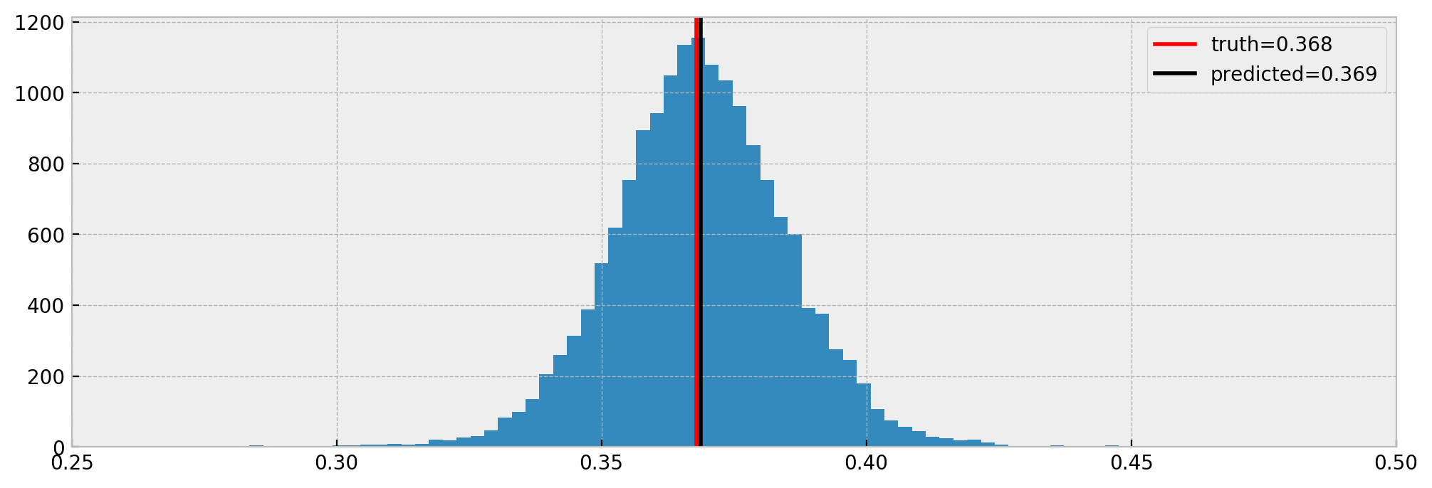
Nice! The model estimated the effect very well again. Note that we have less samples in the histogram, due to NaNs. Nevertheless, it is a cool result and shows that ForestEmbeddingsCounterfactual can work with confounded data.
Diagnosis and criticism
Now things get interesting. Let us check how our 2D embedding changes with the confounding effect:
# getting embedding from data
reduced_embed = fecf.get_umap_embedding(X)
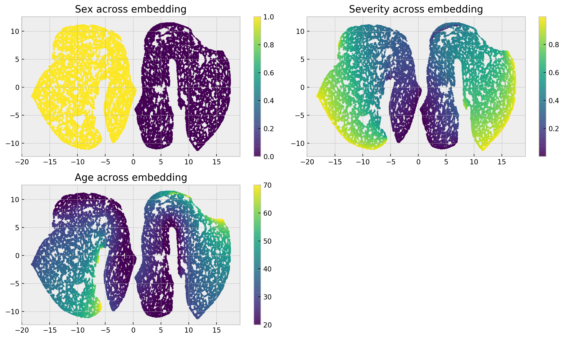
The distribution of explanatory variables across the embedding gets a little bit different. Sex still breaks the embedding into two separate clusters, but severity is now distributed in a up-down gradient inside each cluster and age follows a left-right gradient. The gradients are still smooth enough such that we can be confident that at each local neighborhood individuals are very similar.
Let us have a look at the outcomes and treatment assignments:
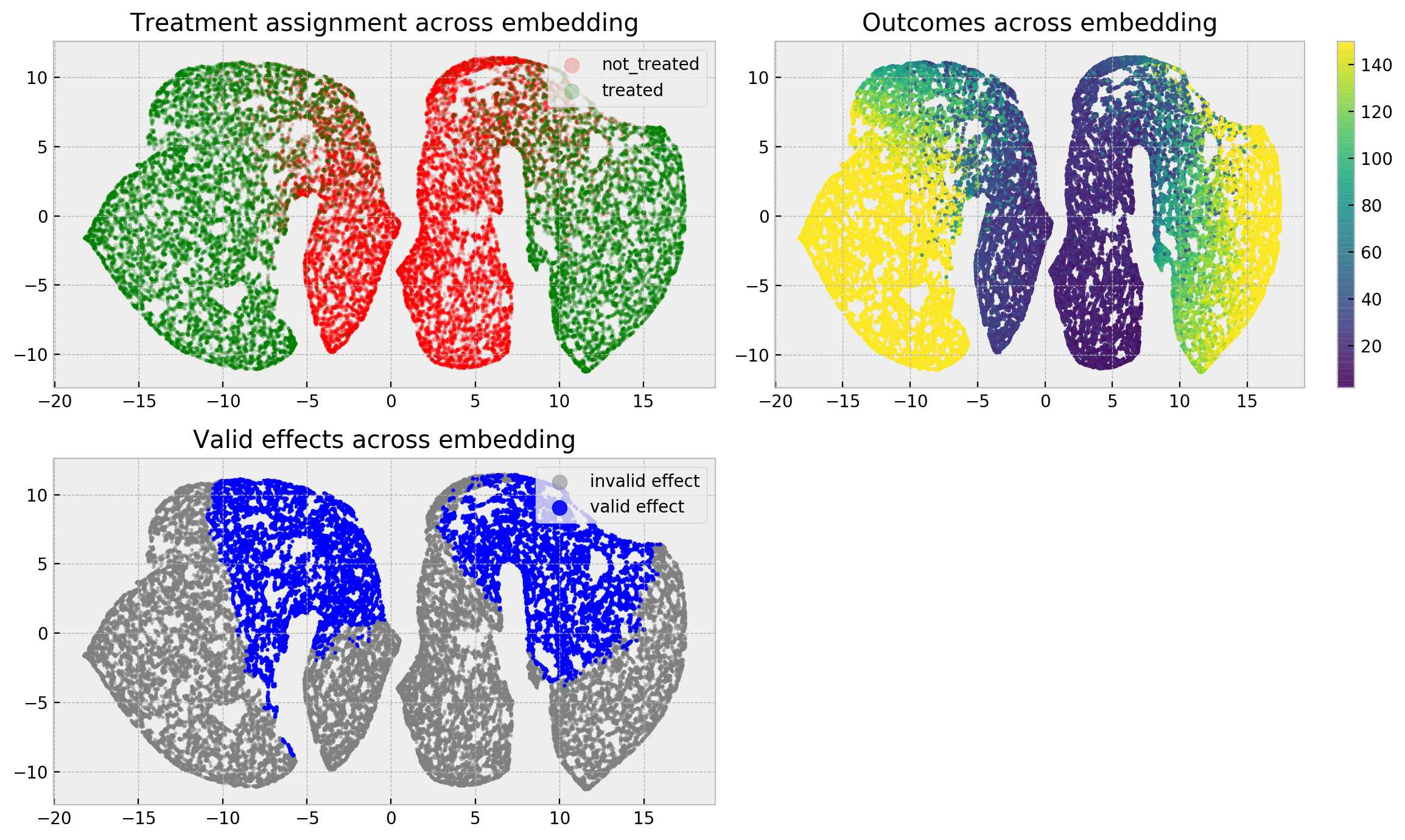
The effect of confounding gets very clear at this point. At the upper left-hand side, we can see that except for a small region at the center of our clusters, there’s no mix of treated and untreated individuals. This lack of mixing makes difficult to estimate counterfactuals, as there’s no similar individuals with different treatment assigments. This makes a lot of the effects invalid, as we see in the lower left-hand side. However, the lack of mixing also made the outcomes more predictable, as we can see in the right-hand side (the embedding is very homogenoeous with respect to the outcome).
If you backtrack a little bit, you’ll notice that we can only predict counterfactuals for people of average severity! That’s why I really like using embeddings for explaining models: they are a quick and visual diagnosis of what your model learned, and can be used to extract knowledge from it for a lot of purposes including causal inference.
And again, if you want to dive deeper just use .explain(). In this case, we query for an individual with high severity and our comparables only have people who were treated, making inference not feasible:
# our test sample
test_sample = X.query('severity > 0.95').iloc[[0]]
print(df_to_markdown(test_sample))
| sex | age | severity |
|---|---|---|
| 0 | 43 | 0.95 |
# running explanation
comparables_table = fecf.explain(test_sample)

# showing comparables table
print(comparables_table['W'].value_counts())
print(df_to_markdown(comparables_table.groupby('W').head(5).sort_values('W').reset_index()))
| index | sex | age | severity | W | y |
|---|---|---|---|---|---|
| 26 | 0 | 43 | 0.95 | 1 | 197 |
| 6526 | 0 | 43 | 0.95 | 1 | 207 |
| 36582 | 0 | 43 | 0.95 | 1 | 211 |
| 21053 | 0 | 43 | 0.96 | 1 | 163 |
| 38484 | 0 | 44 | 0.95 | 1 | 189 |
I hope you liked the tutorial and will use cfml_tools for your causal inference problems soon!