Bayesian deep learning has been received a lot of attention in the ML community, with many attempts to quantify uncertainty in neural networks. Variational Inference, Monte Carlo Dropout and Bootstrapped Ensembles are some examples of research in this area.
Recently, the paper “Randomized Prior Functions for Deep Reinforcement Learning”, presented at NeurIPS 2018, proposes a simple yet effective model for capturing uncertainty, by building an ensemble of bootsrapped neural networks coupled with randomized prior functions: randomly initialized networks that aim to dictate the model’s behavior in regions of the space where there is no training data.
In this Notebook, I’ll build a simple implementation of this model using keras and show some cool visuals to get an intuitive feel of how it works. This is the first of a series of posts where I’ll explore this model and apply it in some cool use cases.
I’ve made the full code available at this Kaggle Kernel, so if you want to run the code while you read, I recommend going there!
1. Starting with a simple example
To motivate this tutorial with a simple yet effective example, I’ll borrow the following data generating process, shown in this bayesian neural network paper by Blundell et. al (2015):
\[y = x + 0.3 \cdot{} sin(2π(x + \epsilon)) + 0.3 \cdot{} sin(4 \cdot{} \pi \cdot{}(x + \epsilon)) + \epsilon\]where $\epsilon \sim \mathcal{N}(0, 0.02)$ and $x \sim U(0.0,0.5)$:
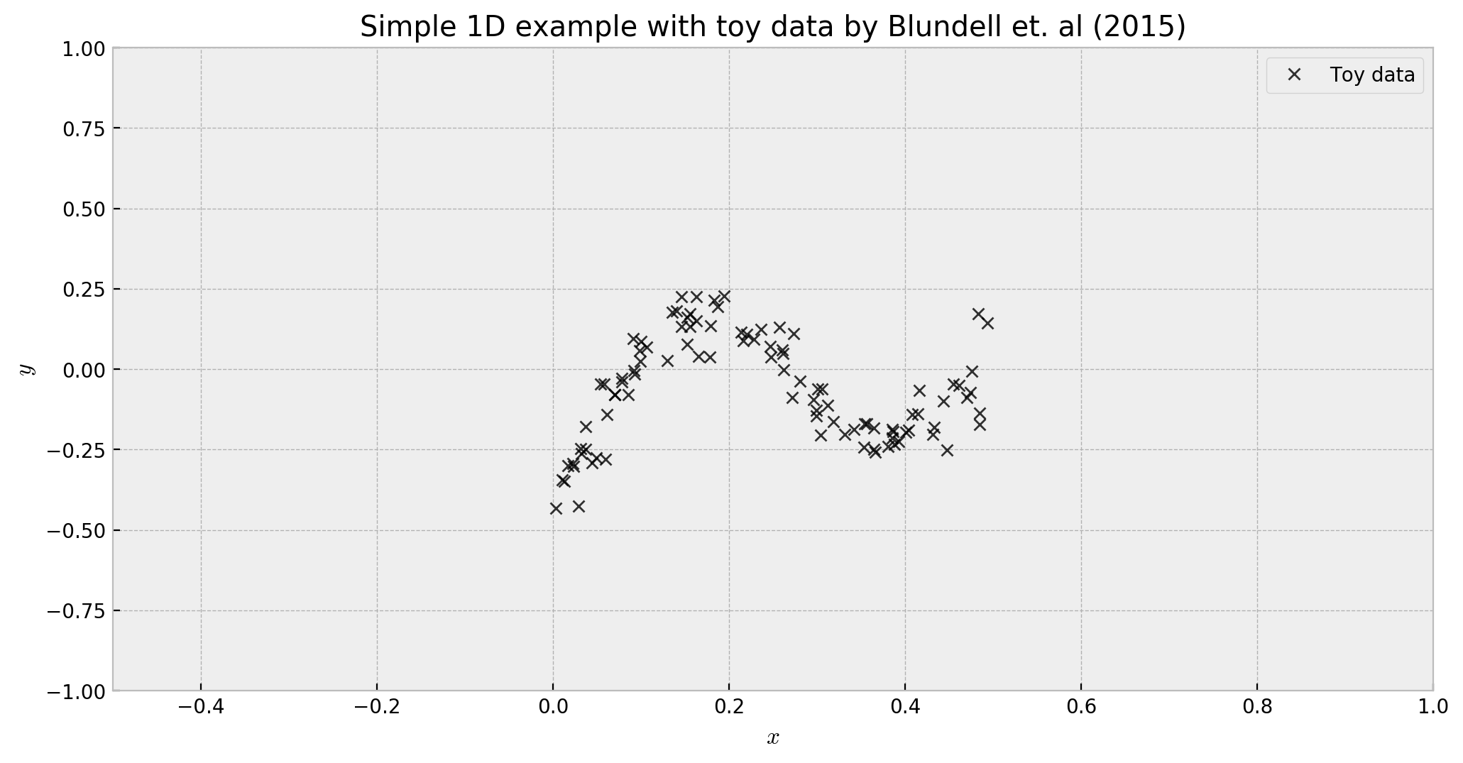
In the example, we have sufficient data only in the interval $[0.0, 0.5]$, but we’re interested in how the model would generalize to other regions of the space. As we move away from the data-rich areas, we expect that the uncertainty will increase: that’s where our randomized prior functions model will help us. Let us build the model step-by-step using this simple dataset as our support.
2. Randomized Prior Functions
To understand what problem randomized prior functions solve, let us recap “Deep Exploration via Bootstrapped DQN”. This approach trains an ensemble of models, each on a bootstrap sample of the data (or a single model with many bootstrapped heads), and approximates uncertainty with the prediction variance across the ensemble. The bootstrap acts as an (actually very good) approximation to the posterior distribution, such that each member of the ensemble can be seen as a sample of the true posterior. Having a good approximation to the posterior gives great benefits for exploration in reinforcement learning: as the agent now knows uncertainty, it can prioritize decisions to maximize both learning and rewards. However, even if the approach works well in practice, there was still something missing: the uncertainty comes only from the data, unlike other bayesian approaches where it also comes from a prior distribution, which would help the agent make decisions in contexts where there is no training data.
To address this shortcoming, Osband et. al proposed a simple yet effective model. It consists of two networks, used in parallel: the trainable network $f$ and the prior network $p$, which are combined to form the final output $Q$, through a scaling factor $\beta$:
\(\large Q = f + \beta\cdot p\)
Let us start with the first part of the model, the prior network. First, we initialize the network with an Input, and a prior_net, for which we enforce fixed weights by setting the parameter trainable to False. The architecture of the network, and the glorot_normal initiatilization have a deep tie to the family of functions that this prior will implement. You’re welcome to try different settings!
# prior network output #
# shared input of the network
net_input = Input(shape=(1,),name='input')
# let us build the prior network with five layers
prior_net = Sequential([Dense(16,'elu',kernel_initializer='glorot_normal',trainable=False),
Dense(16,'elu',kernel_initializer='glorot_normal',trainable=False)],
name='prior_net')(net_input)
# prior network output
prior_output = Dense(1,'linear',kernel_initializer='glorot_normal',
trainable=False, name='prior_out')(prior_net)
# compiling a model for this network
prior_model = Model(inputs=net_input, outputs=prior_output)
# let us score the network and plot the results
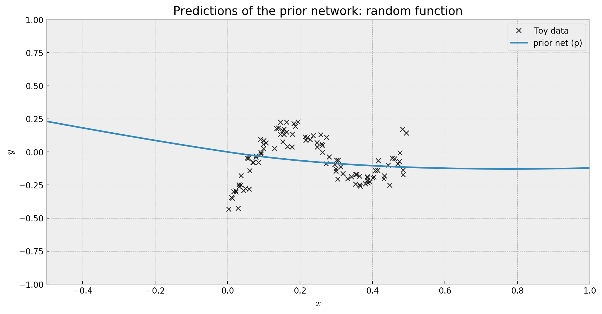
prior_preds = 3 * prior_model.predict(x_grid)
The predictions of this net show that it implements a random function, like we wanted:
The second part of the model is the trainable network, with the same architecture as the prior, but with no fixed weights. It receives the same net_input as the prior.
# adding trainable network #

# trainable network body
trainable_net = Sequential([Dense(16,'elu'),
                            Dense(16,'elu')],
                           name='trainable_net')(net_input)

# trainable network output
trainable_output = Dense(1,'linear',name='trainable_out')(trainable_net)
Trainable and prior interact via an add layer, so the trainable network can optimize its weights conditioned on the prior. We use a Lambda layer to scale the prior output, so we can implement $\beta$ in the add layer.
# using a lambda layer so we can control the weight (beta) of the prior network
prior_scale = Lambda(lambda x: x * 3.0, name='prior_scale')(prior_output)

# lastly, we use a add layer to add both networks together and get Q
add_output = add([trainable_output, prior_scale], name='add')

# defining the model and compiling it
model = Model(inputs=net_input, outputs=add_output)
model.compile(loss='mean_squared_error', optimizer='adam', metrics=['mean_squared_error'])
Let us check the final architecture:
# checking final architecture
from IPython.display import SVG
from keras.utils.vis_utils import model_to_dot

SVG(model_to_dot(model).create(prog='dot', format='svg'))
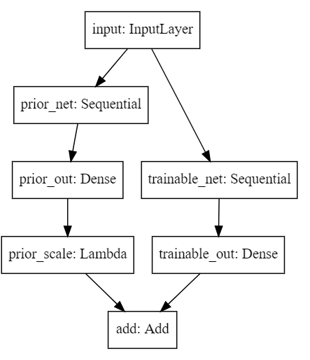
The architecture is actually very simple. It’s like traning two nets in parallel, but in this case, one of them is not trained! For me, this model is the simplest way to be bayesian: you just use vanilla networks, but combined in a smart way.
Let us fit the model, and get the trainable output:
# let us fit the model
model.fit(X, y, epochs=2000, batch_size=100, verbose=0)

# let us get the individual output of the trainable net
trainable_model = Model(inputs=model.input, outputs=model.get_layer('trainable_out').output)
And finally, let us plot prior, trainable and final output together:
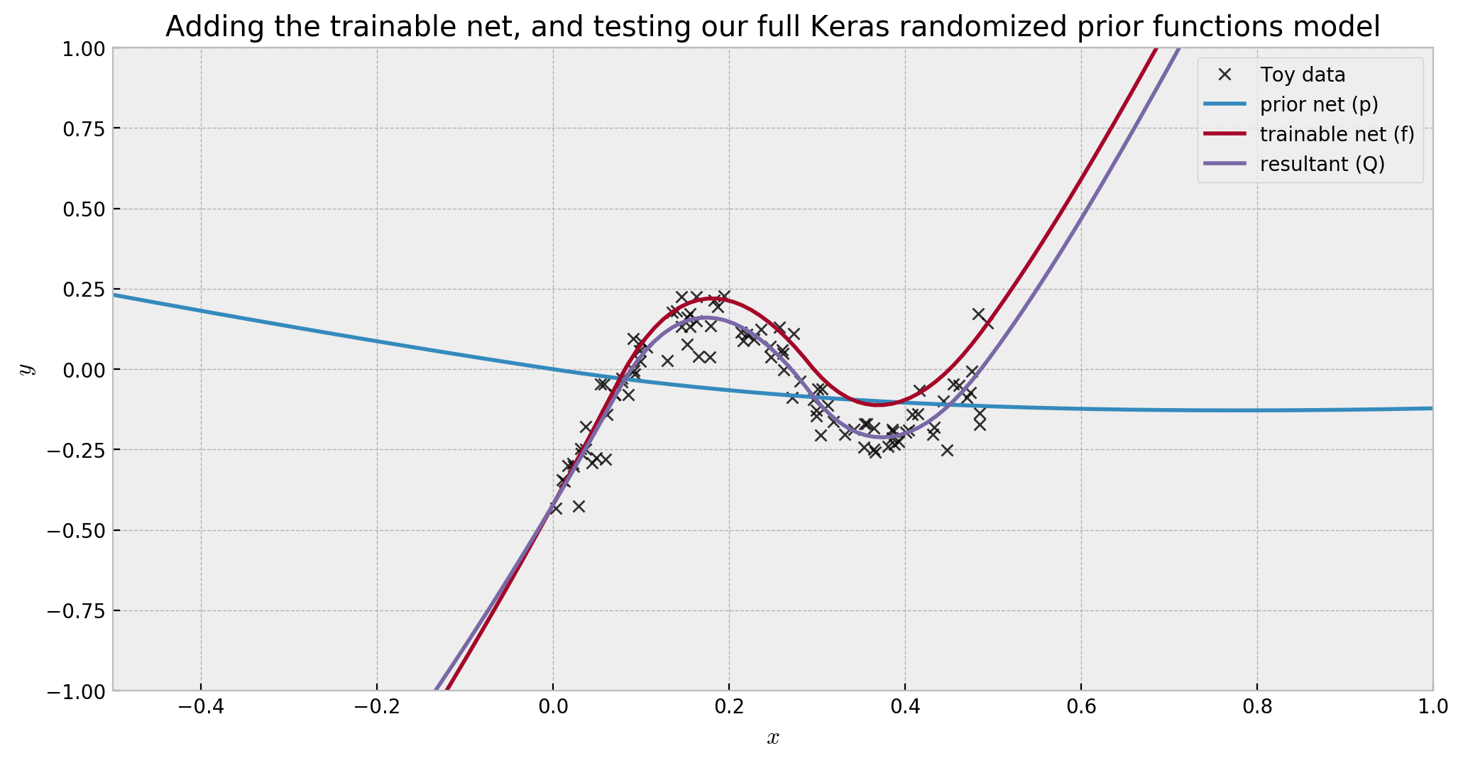
As we can see, the trainable network (dark red) compensated the prior network (blue), reasonably fitting our data (purple). However, in regions away from our data, the prior network will dominate, fulfilling its uncertainty-driver role.
Let us wrap everything up in the function get_randomized_prior_nn below, so that we’re ready to move to the next step: Bootstrapped Ensembles!
# function to get a randomized prior functions model
def get_randomized_prior_nn():

    # shared input of the network
    net_input = Input(shape=(1,), name='input')

    # trainable network body
    trainable_net = Sequential([Dense(16,'elu'),
                                Dense(16,'elu')],
                               name='trainable_net')(net_input)

    # trainable network output
    trainable_output = Dense(1, 'linear', name='trainable_out')(trainable_net)

    # prior network body - we use trainable=False to keep the network output random
    prior_net = Sequential([Dense(16,'elu',kernel_initializer='glorot_normal',trainable=False),
                            Dense(16,'elu',kernel_initializer='glorot_normal',trainable=False)],
                           name='prior_net')(net_input)

    # prior network output
    prior_output = Dense(1, 'linear', kernel_initializer='glorot_normal', trainable=False, name='prior_out')(prior_net)

    # using a lambda layer so we can control the weight (beta) of the prior network
    prior_output = Lambda(lambda x: x * 3.0, name='prior_scale')(prior_output)

    # lastly, we use a add layer to add both networks together and get Q
    add_output = add([trainable_output, prior_output], name='add')

    # defining the model and compiling it
    model = Model(inputs=net_input, outputs=add_output)
    model.compile(loss='mean_squared_error', optimizer='adam', metrics=['mean_squared_error'])

    # returning the model
    return model
3. Bootstrapped Ensembles
Although already very cool, our model is not complete yet, as with only one network we just have one sample of the posterior distribution. We need to generate more samples if we want to have a good approximation of the true posterior. This is where a bootstrapped ensemble comes in, and it’s actually very simple to build it.
As we have the generator function get_randomized_prior_nn for our model, we can just generate many versions of it and train them using the BaggingRegressor from sklearn. This effectively performs the bootstrapping we need, in just a few lines of code:
# wrapping our base model around a sklearn estimator
base_model = KerasRegressor(build_fn=get_randomized_prior_nn,
                            epochs=3000, batch_size=100, verbose=0)

# create a bagged ensemble of 10 base models
bag = BaggingRegressor(base_estimator=base_model, n_estimators=9, verbose=2)
We fit the ensemble just like any other sklearn model.
# fitting the ensemble
bag.fit(X, y.ravel())
After fitting our ensemble, we can check what the trainable, prior and resultant networks output looks like, just as we did before:
# individual predictions on the grid of values
y_grid = np.array([e.predict(x_grid.reshape(-1,1)) for e in bag.estimators_]).T
trainable_grid = np.array([Model(inputs=e.model.input,outputs=e.model.get_layer('trainable_out').output).predict(x_grid.reshape(-1,1)) for e in bag.estimators_]).T
prior_grid = np.array([Model(inputs=e.model.input,outputs=e.model.get_layer('prior_scale').output).predict(x_grid.reshape(-1,1)) for e in bag.estimators_]).T
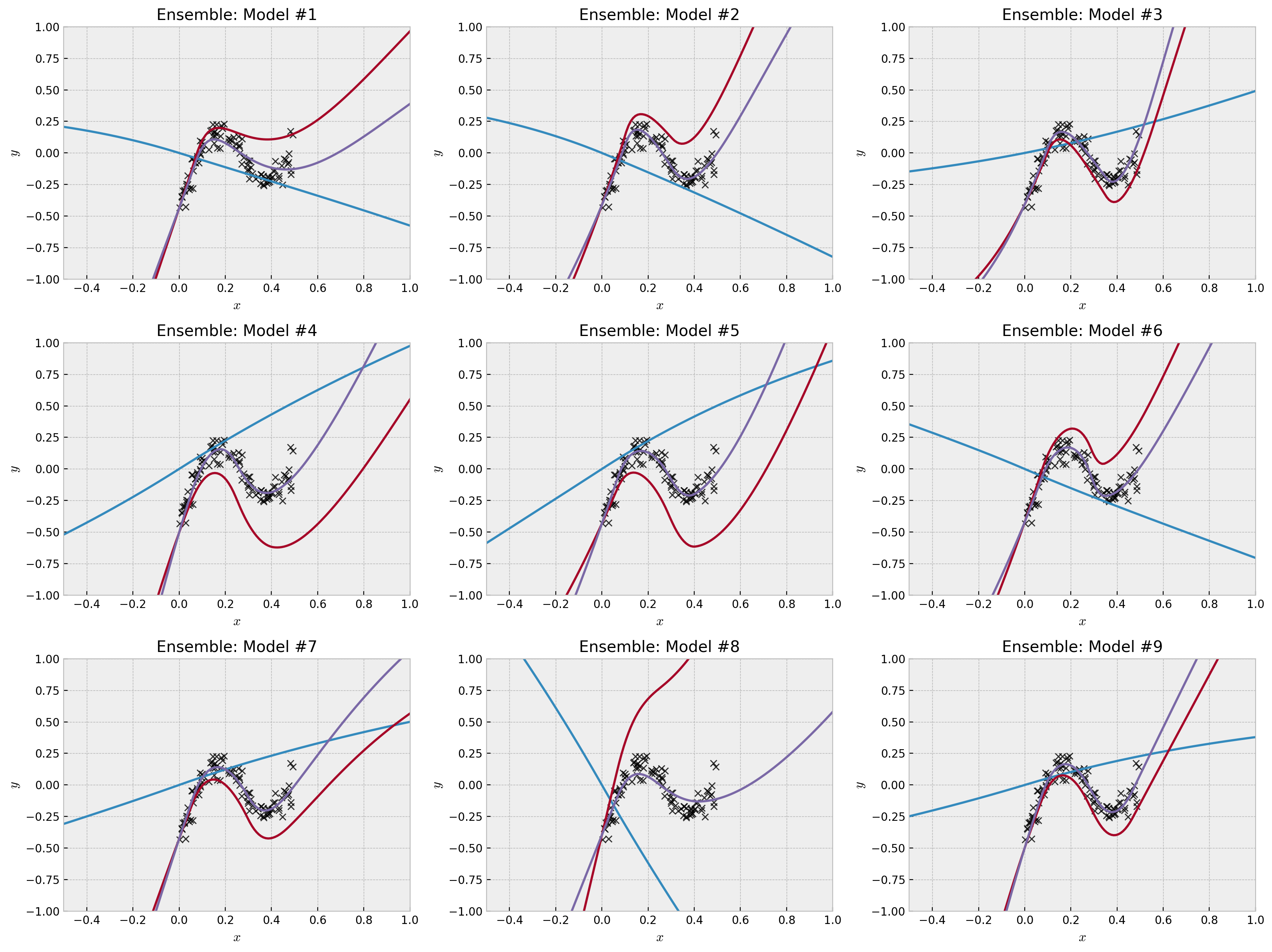
We can see how the prior network affects the final predictions, pushing model diversity into the ensemble. How this model diversity influences the final predictions?
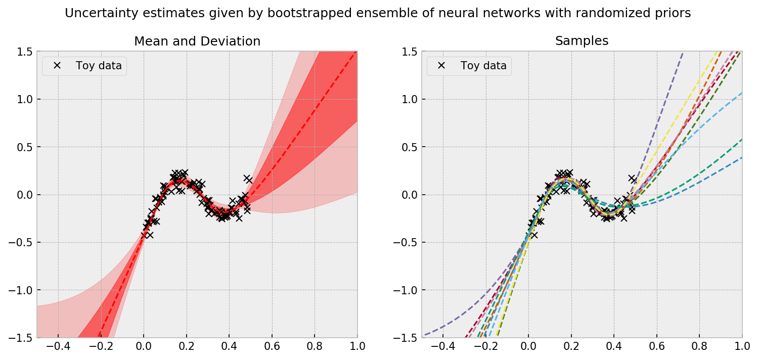
We can see that in data rich regions, we have strong agreement across members of the ensemble. However, the further we are from the data, disagreement and larger uncertainties arise. The uncertainty estimate is principled; in the paper, the authors show (for the linear case) that each member of the ensemble is actually a sample from the real posterior. To use the model to make decisions, a simple and good policy is to randomly select one member of the ensemble and let it take the wheel for the next round or episode (which is equivalent to Thompson Sampling).
4. Effect of prior and bootstrapping
This model is really cool, but one might ask: what is actually driving uncertainty? The bootstrap? The prior? The neural network optimization process, with many local optima?
In order to draft some answers to these questions, let us conclude this post running three more models, comparing them to the full randomized prior functions model:
- Ensemble of networks with prior, but with bootstrapping turned off
- Ensemble of regular networks (no prior), but with bootstrapping turned on
- Ensemble of regular networks, and boostrapping turned off (no prior, and no bootstrap)
We start by defining a function get_regular_nn to implement a regular NN to use in models (2) and (3). I’ll reuse the implementation of the trainable network:
# function to get a randomized prior functions model
def get_regular_nn():

    # shared input of the network
    net_input = Input(shape=(1,), name='input')

    # trainable network body
    trainable_net = Sequential([Dense(16, 'elu'),
                                Dense(16, 'elu')],
                               name='trainable_net')(net_input)

    # trainable network output
    trainable_output = Dense(1, activation='linear', name='trainable_out')(trainable_net)

    # defining the model and compiling it
    model = Model(inputs=net_input, outputs=trainable_output)
    model.compile(loss='mean_squared_error', optimizer='adam', metrics=['mean_squared_error'])

    # returning the model
    return model
Then, we build the models. For models with no bootstrap, we set the option bootstrap to False in BaggingRegressor. For models with no prior, we use get_regular_nn instead of get_randomized_prior_nn for the build_fn option.
# wrapping our base models around a sklearn estimator
base_rpf = KerasRegressor(build_fn=get_randomized_prior_nn,
                          epochs=3000, batch_size=100, verbose=0)
base_reg = KerasRegressor(build_fn=get_regular_nn,
                          epochs=3000, batch_size=100, verbose=0)

# our models
prior_but_no_boostrapping = BaggingRegressor(base_rpf, n_estimators=9, bootstrap=False)
bootstrapping_but_no_prior = BaggingRegressor(base_reg, n_estimators=9)
no_prior_and_no_boostrapping = BaggingRegressor(base_reg, n_estimators=9, bootstrap=False)

# fitting the models
prior_but_no_boostrapping.fit(X, y.ravel())
bootstrapping_but_no_prior.fit(X, y.ravel())
no_prior_and_no_boostrapping.fit(X, y.ravel())

# individual predictions on the grid of values
y_grid = np.array([e.predict(x_grid.reshape(-1,1)) for e in bag.estimators_]).T
y_grid_1 = np.array([e.predict(x_grid.reshape(-1,1)) for e in prior_but_no_boostrapping.estimators_]).T
y_grid_2 = np.array([e.predict(x_grid.reshape(-1,1)) for e in bootstrapping_but_no_prior.estimators_]).T
y_grid_3 = np.array([e.predict(x_grid.reshape(-1,1)) for e in no_prior_and_no_boostrapping.estimators_]).T
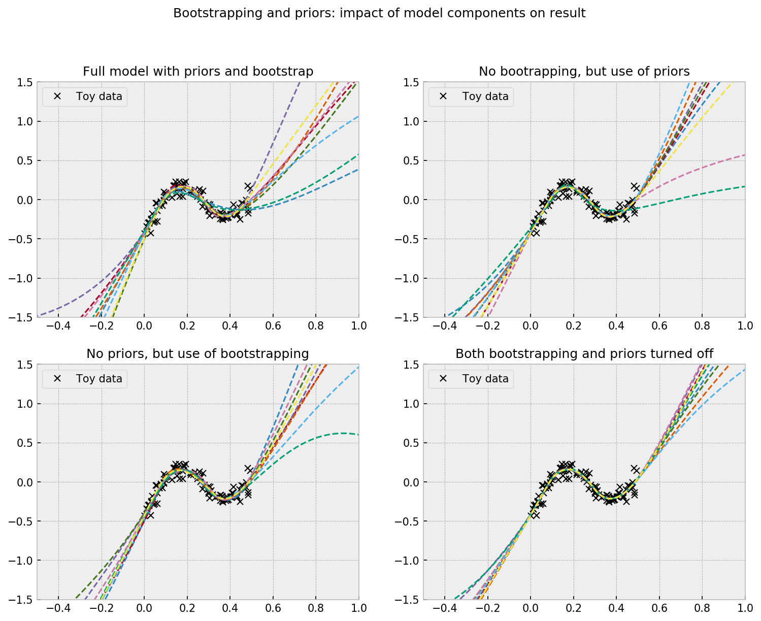
The plot shows the impact of priors and bootstrapping as drivers of uncertainty. At the upper left corner we see the full model, which shows a wide disagreement between ensemble members (uncertainty) on regions with no data. Generally, turning bootstrapping off will reduce uncertainty the most (upper right corner), as opposed to turning priors off (lower left corner), but it can vary a bit across different seeds. With both bootstrapping and priors off, there’s still a little disagreement between ensemble members due to random initialization of weights, but is a lot less compared to the other models.
5. Conclusion
In this tutorial, we built one of the state-of-the-art models for deep bayesian learning: a neural network with a randomized prior function, in a simple keras implementation. The model is pretty cool and does a good job in estimating uncertainty. To further test the model and apply it to different areas, I’ll try to apply it in a bandit problem next. Stay tuned!
Hope you liked the tutorial!!!! Any feedback is appreciated!
See you soon!