Thompson Sampling is a very simple yet effective method to addressing the exploration-exploitation dilemma in reinforcement/online learning. In this series of posts, I’ll introduce some applications of Thompson Sampling in simple examples, trying to show some cool visuals along the way. All the code can be found on my GitHub page here.
In this post, we frame the hyperparameter optimization problem (a theme that is much explored by the AutoML community) as a bandit problem, and use Gaussian Processes to solve it.
Optimization of non-differentiable and non-convex functions
Before we dive into actual hyperparameter optimization, let us illustrate the problem with a simpler example, but rather challenging: a 1D cut of the Ackley function.
# defining the function. At y=0 to get a 1D cut at the origin
def ackley_1d(x, y=0):

    # the formula is rather large
    out = (-20*np.exp(-0.2*np.sqrt(0.5*(x**2 + y**2)))
           - np.exp(0.5*(np.cos(2*np.pi*x) + np.cos(2*np.pi*y)))
           + np.e + 20)

    # returning
    return out
The resulting function determines the following plot:
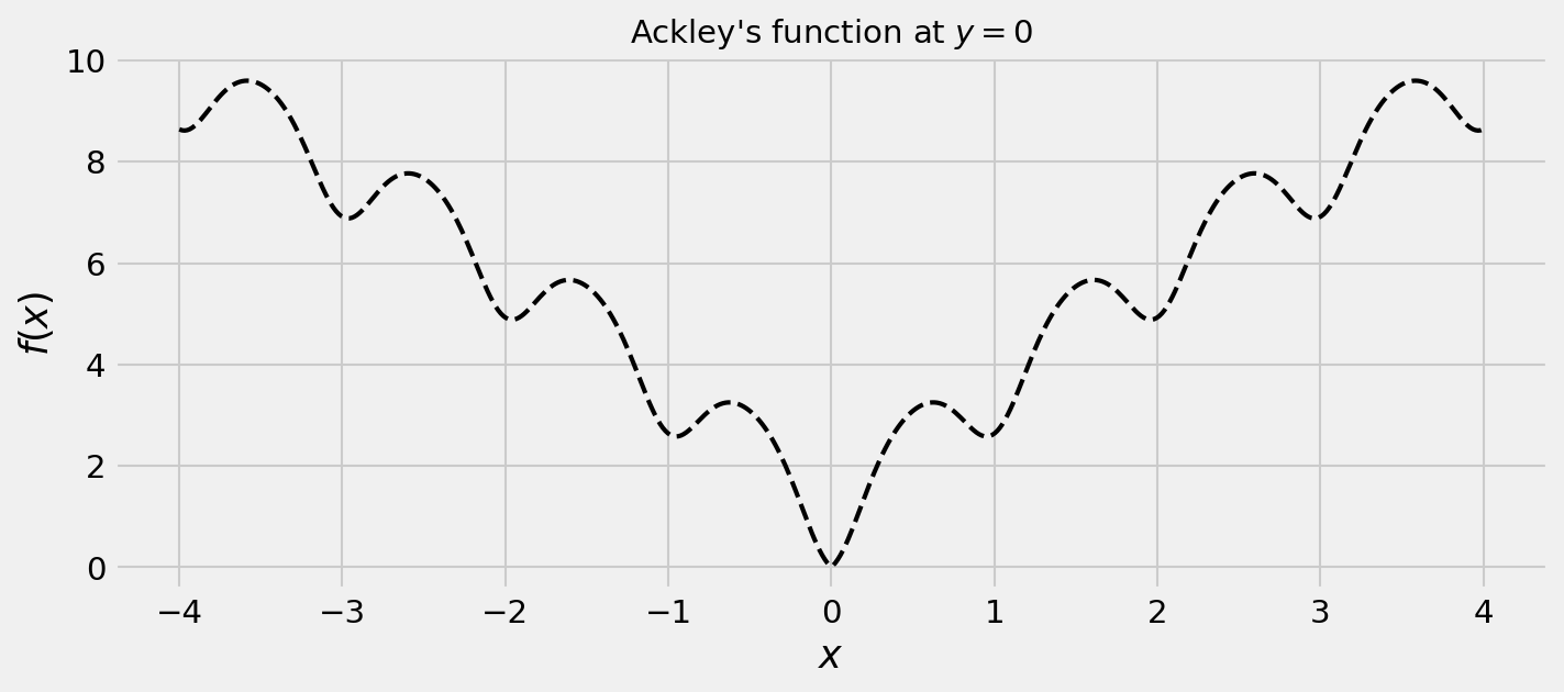
The Ackley’s function has a lot of local minima, therefore it’s not convex. This makes harder for us to achive our goal to minimize it. Furthermore, we will add a twist: we will not make the function’s derivatives available. This way, we’re closer to a real hyperparameter optimization problem.
First, we need a method that can approximate this function and also calculate the uncertainty over the approximation. Gaussian Processes are a elegant way to achieving these goals.
Gaussian Processes
Gaussian Processes are supervised learning methods that are non-parametric, unlike the Bayesian Logistic Regression we’ve seen earlier. Instead of trying to learn a posterior distribution over the parameters of a function $f(x) = \theta_0 + \theta_1 \cdot x + \epsilon$ we learn a posterior distribution over all the functions.
We specify how smooth the functions will be through covariance functions (kernels), which calculate the similarity between samples. If we enforce that similar points in input space produce similar outputs, we have a smooth function. I recommend this tutorial and this for further reading. Also, these classes are very nice.
Using sklearn we can easily fit a GP to a few samples of our target function:
# let us draw 20 random samples of the Ackley's function
x_observed = np.random.uniform(-4, 4, 20)
y_observed = ackley_1d(x_observed)

# let us use the Matern kernel
K = 1.0 * Matern(length_scale=1.0, length_scale_bounds=(1e-1, 10.0), nu=1.5)

# instance of GP
gp = GaussianProcessRegressor(kernel=K)

# fitting the GP
gp.fit(x_observed.reshape(-1,1), y_observed)
When we call the .fit() method, the GP infers a posterior distribution over functions, given the smoothness constraints given by the kernel. The gp object can return the posterior means and variances for a grid in our search space:
# let us check the learned model over all of the input space
X_ = np.linspace(-4, 4, 500)
y_mean, y_std = gp.predict(X_.reshape(-1,1), return_std=True)
Plotting these values, we get the following figure:
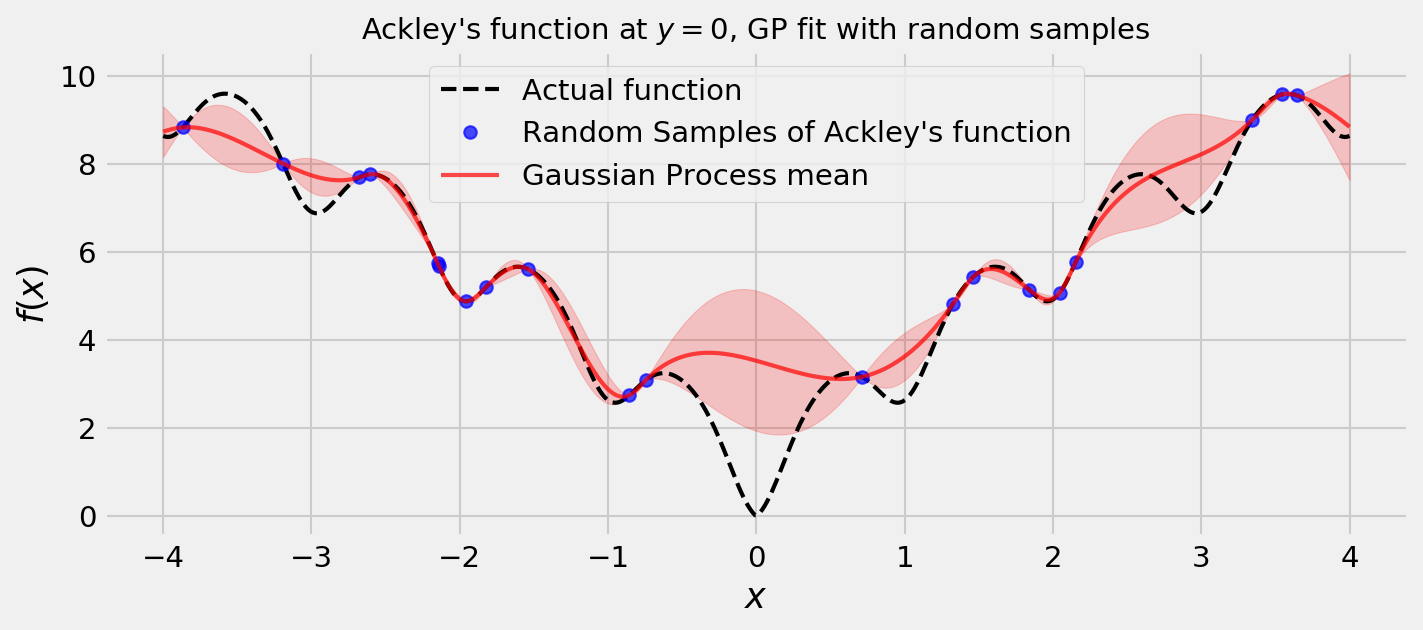
Cool! The uncertainties seem reasonable. We can also draw some samples from the posterior. Remember: samples from a GP are functions themselves!
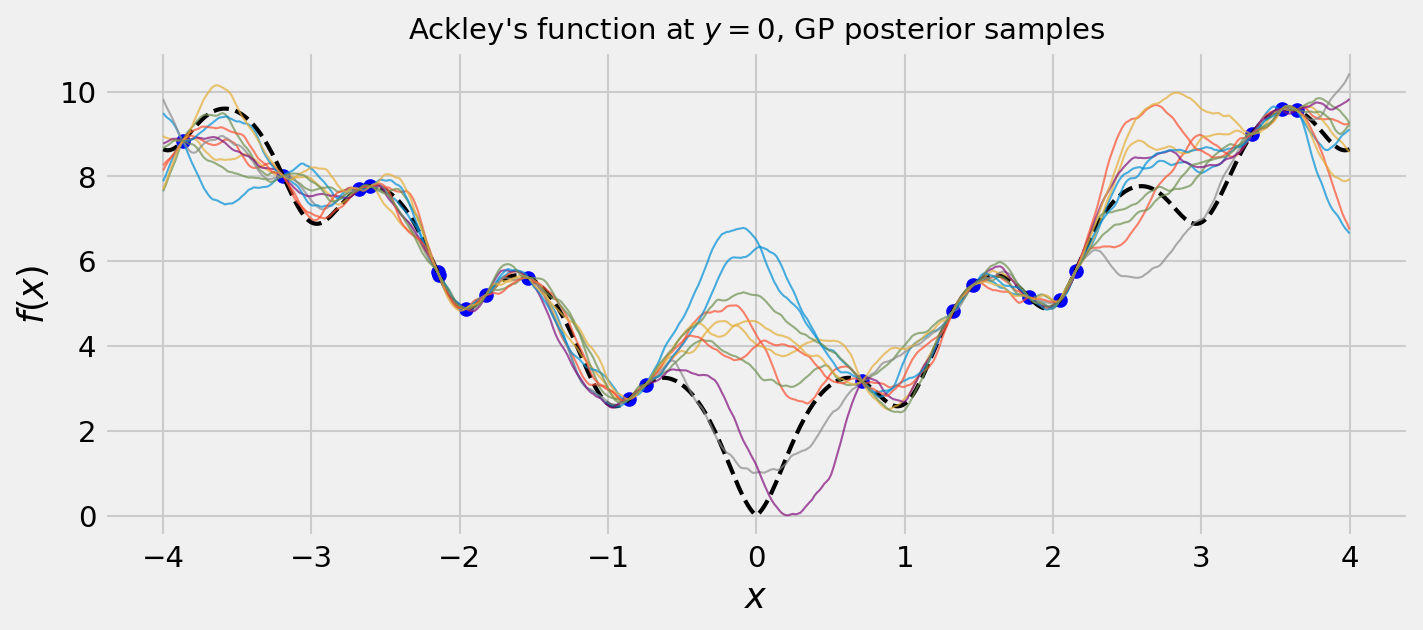
We can see that our samples seem very plausible. This is due to a good choice of kernel. The Matérn kernel in my experience fares well in most cases. Feel free to get the code in my GitHub and try others!
Thompson Sampling for a GP
Ok. So we learned how a GP works, and how we can draw functions from the posterior distribution it learns. So, now, how do we use Thompson Sampling with it? It’s very simple:
- Fit the GP to the observations we have
- Draw one sample (a function) from the posterior
- Greedily choose the next point with respect to the sample
The randomness of Thompson Sampling comes from the posterior sample. After we have it, we can just use its minimum as our next point. Let us implement this.
# our TS-GP optimizer
class ThompsonSamplingGP:

    # initialization
    def __init__(self, n_random_draws, objective, x_bounds, interval_resolution=1000):

        # number of random samples before starting the optimization
        self.n_random_draws = n_random_draws

        # the objective is the function we're trying to optimize
        self.objective = objective

        # the bounds tell us the interval of x we can work
        self.bounds = x_bounds

        # interval resolution is defined as how many points we will use to
        # represent the posterior sample
        # we also define the x grid
        self.interval_resolution = interval_resolution
        self.X_grid = np.linspace(self.bounds[0], self.bounds[1], self.interval_resolution)

        # also initializing our design matrix and target variable
        self.X = np.array([]); self.y = np.array([])

    # fitting process
    def fit(self, X, y):

        # let us use the Matern kernel
        K = 1.0 * Matern(length_scale=1.0, length_scale_bounds=(1e-1, 10.0), nu=1.5)

        # instance of GP
        gp = GaussianProcessRegressor(kernel=K)

        # fitting the GP
        gp.fit(X, y)

        # return the fitted model
        return gp

    # process of choosing next point
    def choose_next_sample(self):

        # if we do not have enough samples, sample randomly from bounds
        if self.X.shape[0] < self.n_random_draws:
            next_sample = np.random.uniform(self.bounds[0], self.bounds[1],1)[0]

        # if we do, we fit the GP and choose the next point based on the posterior draw minimum
        else:
            # 1. Fit the GP to the observations we have
            self.gp = self.fit(self.X.reshape(-1,1), self.y)

            # 2. Draw one sample (a function) from the posterior
            posterior_sample = self.gp.sample_y(self.X_grid.reshape(-1,1), 1).T[0]

            # 3. Choose next point as the optimum of the sample
            which_min = np.argmin(posterior_sample)
            next_sample = self.X_grid[which_min]

            # let us also get the std from the posterior, for visualization purposes
            posterior_mean, posterior_std = self.gp.predict(self.X_grid.reshape(-1,1), return_std=True)

        # let us observe the objective and append this new data to our X and y
        next_observation = self.objective(next_sample)
        self.X = np.append(self.X, next_sample)
        self.y = np.append(self.y, next_observation)

        # return everything if possible
        try:
            # returning values of interest
            return self.X, self.y, self.X_grid, posterior_sample, posterior_mean, posterior_std

        # if not, return whats possible to return
        except:
            return (self.X, self.y, self.X_grid, np.array([np.mean(self.y)]*self.interval_resolution),
                    np.array([np.mean(self.y)]*self.interval_resolution), np.array([0]*self.interval_resolution))
With this implementation, we can run one episode telling the algorithm to find the minimum of the Ackley’s function. The results follow. We plot the predictive variance of the GP and the posterior sample used to choose the next point in each round.
For most of the times I ran this code, I observed a good balance of exploration and exploitation. As we get closer to the global minimum, the uncertainty is reduced, and the algorithm concentrates its efforts where it finds more promising. For the other zones, we may have a large uncertainty, but this is fine since even with this uncertainty there’s not a significant chance of improvement.
Hyperparameter optimization
Now we face the real challenge of hyperparameter optimization. We’re going to perform the same optimization methodology we did before, but with the difference that our objective function is the result of a cross-validation experiment and our $x$ is a hyperparameter of an algorithm.
Let us try tuning a Lasso to solve the Diabetes dataset from the UCI repository. It’s very easy to load the data using sklearn:
# loading the data
diabetes = datasets.load_diabetes()
X = diabetes.data[:150]
y = diabetes.target[:150]
We define the objetive function as a class, in order to store the data. A function evaluation is an execution of a cross validation loop returning the validation $R^2$ as the objective value. As our algorithm is programmed to minimize things, we return the negative of the $R^2$ value.
# now let us devise our objective function
class LassoDiabetesObjective:

    # initialization with data
    def __init__(self, X_train, y_train):

        # storing
        self.X_train = X_train
        self.y_train = y_train

    # validation experiment
    def validation_experiment(self, exp_alpha):

        # instance of svm
        lasso = Lasso(alpha=10**exp_alpha)

        # instance of CV scheme
        k_fold = KFold(n_splits=3, shuffle=True, random_state=20171026)

        # fitting on train
        preds = cross_val_predict(lasso, self.X_train, self.y_train, cv=k_fold)

        # validation accuraccy
        cv_r2 = r2_score(self.y_train, preds)

        # returning negative as our function minimizes the objective
        return -cv_r2
The following animation shows the optimization running over some rounds:
In most of my runs, the optimization was actually very easy for our TS-GP methodology. Again, feel free to grab the Notebook at my GitHub page to expand the code to the multivariate case, where we have many decision variables and our TS-GP will be even more useful.
Conclusion
In this notebook, we used a model which computes a posterior distribution not on parameters, but functions, given the data. This way, we can sample these functions and apply Thompson Sampling to address exploration/exploitation for optimizing non-convex, non-differentiable functions, like a hyperparameter tuning problem.
For further information about research in hyperparameter tuning (and a little more!), refer to the AutoML website. Not limited to just hyperparameter tuning, research in the field proposes a completely automatic model building and selection process, with every moving part being optimized by Bayesian methods and others.