Thompson Sampling is a very simple yet effective method to addressing the exploration-exploitation dilemma in reinforcement/online learning. In this series of posts, I’ll introduce some applications of Thompson Sampling in simple examples, trying to show some cool visuals along the way. All the code can be found on my GitHub page here.
In this post, we explore more advanced algorithms, starting with a simple trial to get uncertainties out of Random Forests and then moving to Bootstrapped Neural Networks. We use these methods to solve the “Mushroom” bandit, a contextual bandit game where the agent must decide, from a bucket of edible and poisonous mushrooms, which ones to eat.
Solving the Mushroom Bandit
In this notebook, we’ll run an experiment inspired by the paper Weight Uncertainty in Neural Networks (Blundell et. al, 2015), the Mushroom bandit. In this setting, we use the Mushroom dataset from UCI to simulate a bandit-like game, in order to test some Thompson Sampling-inspired algorithms that try to address the exploration-exploitation tradeoff. Particularly, we will test two interesting ideas:
Bootstrapped Neural Networks: based on Bootstrapped DQN, a proven method for deep exploration in reinforcement learning, presented by Osband et. al. (2016). Here, we do not have a full RL setting, so we call it a Bootstrapped Neural Network, rather than a Bootstrapped DQN.
Sampling from a Random Forest: let us try to use the individual tree predictions of a Random Forest to build uncertainty estimates for our game.
We will also test the greedy counterparts of these ideas, a regular neural network and a regular Random Forest.
Test with toy data
Let us first run our models with simple toy data to check uncertainty estimates.
Generating the data
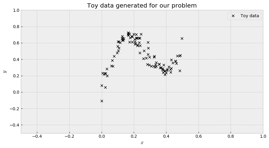
We will use the formula given by the paper Weight Uncertainty in Neural Networks to generate the data:
\[y = x + 0.3 \cdot{} sin(2π(x + \epsilon)) + 0.3 \cdot{} sin(4 \cdot{} \pi \cdot{}(x + \epsilon)) + \epsilon\]where $\epsilon \sim \mathcal{N}(0, 0.02)$. We take a hundred $x$ samples from an uniform distribution $\mathcal{U}(0, 0.5)$. This results in the following plot:
Random Forest
Let us start with the simpler model, a Random Forest. What we will try to do is randomize the forest’s output, by sampling sets of decision trees and averaging their predictions. The following code accomplishes that, drawing 20 samples of our approximate posterior distribution.
# instance of RF
et = ExtraTreesRegressor(n_estimators=100, min_samples_leaf=2)

# let us fit it to the data
et.fit(x.reshape(-1,1),y)

# let us generate data to check the fit
x_grid = np.linspace(-0.5, 1.0, 200).reshape(-1,1)

# number of samples from the forest
N_SAMPLES = 20

# let us get the predictions of four trees at a time
tree_samples = [np.random.choice(et.estimators_, 4) for i in range(N_SAMPLES)]

# let us predict with these guys
y_grid = np.array([np.array([e.predict(x_grid) for e in np.random.choice(et.estimators_, 2)]).mean(axis=0) for tree_sample in tree_samples])
The sampling procedure results in the following plot:
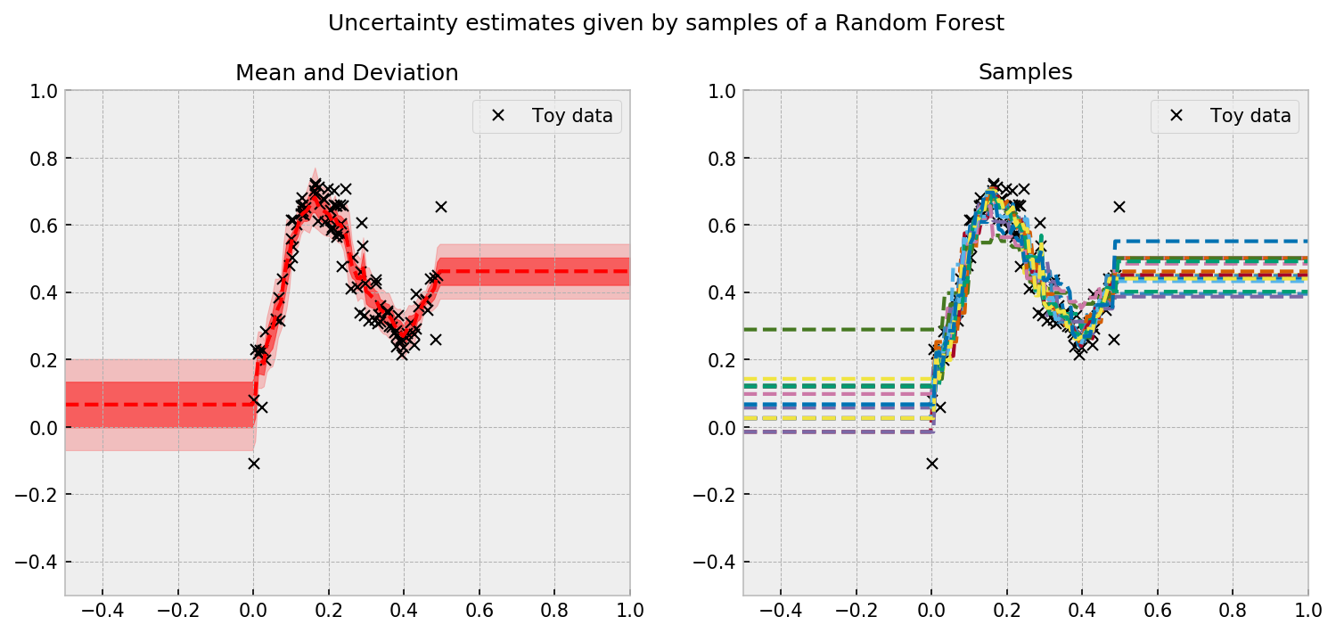
The uncertainty estimates concentrate where there is more data, which is a good sign. However, uncertainties do not increase as we get distant from the samples. This may be due to the rule-based learning procedure of RF’s, which prevents them from extrapolating.
Bootstrapped Neural Network
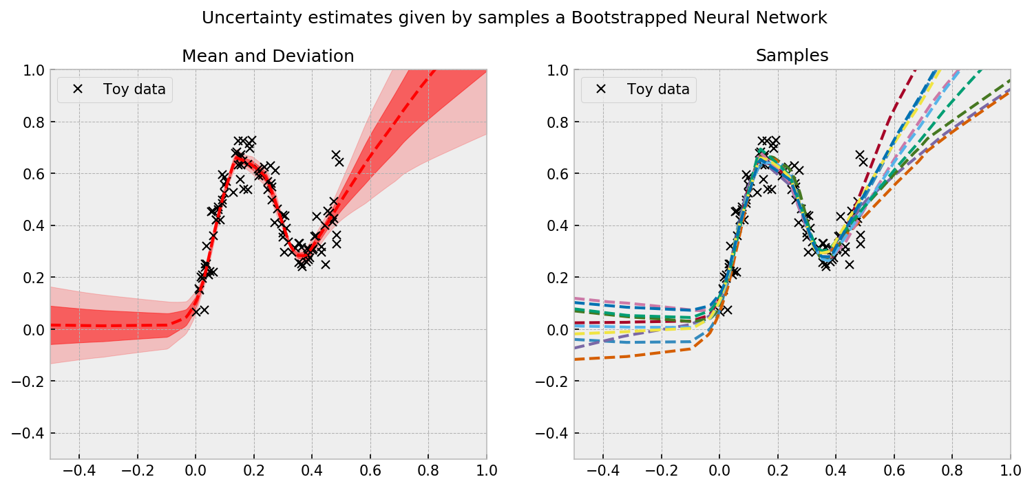
Let us check the uncertainty estimates produced by our Bootstrapped NN. As introduced by Osband et. al. (2016), we will train a network with a shared layer and many bootstrapped heads, which will diverge a little bit on their predictions. This divergence will drive efficient exploration and will give us reasonable uncertainty estimates.
I made a quick and dirty implementation of this model on Keras, but it’s far from ideal. Here, I generate the bootstrap samples at model compile time, and return $N$ bootstrapped samples of the training dataset, consuming a lot of memory. The model trains on 10 different inputs and outputs.
# defining the model #

# shared network
shared_net = Sequential([Dense(1, activation='linear', input_dim=1),
                         Dense(16, activation='relu'),
                         Dense(16, activation='relu'),
                         Dense(16, activation='relu')])


# bootstrap rate and number of heads
BOOTSTRAP_RATE = 1.00
N_HEADS = 10

# initializing lists
inputs = []
heads = []
x_btrap = []
y_btrap = []

# loop for creating heads and sampled data points
for i in range(N_HEADS):

    # deciding sample of data points
    sample_idx = np.random.choice(range(x.shape[0]), int(x.shape[0]*BOOTSTRAP_RATE), True)

    # defining the heads in the graph
    input_temp = Input(shape=(1,))
    shared_temp = shared_net(input_temp)
    head_temp = Dense(16, activation='relu')(shared_temp)
    heads.append(Dense(1, activation='linear')(head_temp))
    inputs.append(input_temp)

    # defining data
    x_btrap.append(x[sample_idx])
    y_btrap.append(y[sample_idx])

# defining the model and plotting it
model = Model(inputs=inputs, outputs=heads)
plot_model(model)

# compiling
model.compile(loss='mean_squared_error', optimizer='adam', metrics=['mean_squared_error'])

# fitting the model
model.fit(x_btrap, y_btrap, epochs=500, batch_size=64, verbose=0);
Even with my dirty code, the results are beautiful. We can see a reasonable uncertainty estimate given by the individual predictions of the bootstrapped heads:
We are now ready to play the Mushroom bandit game!
The Mushroom bandit
The game is set up as follows:
- The agent is initialized with 50 random mushrooms and if they’re edible or poisonous
- At each round, the agent is presented with all the mushrooms which were not already eaten.
- The agent ranks the mushrooms, with the most edible mushroom at the top.
- The agent eats the top $k$ mushrooms and receives feedback. The agent reward is the actual observation.
Here’s my code to implement the game:
# coding a class for this
class MushroomBandit:

    # initializing
    def __init__(self, X, y):

        # storing the initialization
        self.X = X; self.y = y

        # let us keep eaten and not eaten mushrooms as well
        self.X_not_eaten = X.copy()
        self.y_not_eaten = y.copy()
        self.X_eaten = pd.DataFrame()
        self.y_eaten = pd.Series()

    # function to show not eaten mushrooms
    def get_not_eaten(self):
        return self.X_not_eaten

    # function to show eaten mushrrooms
    def get_eaten(self):
        return self.X_eaten, self.y_eaten

    # function to get which mushrooms will be eaten
    def eat_mushrooms(self, mushroom_idx):

        # get feedback
        feedback = self.y_not_eaten.loc[mushroom_idx].copy()

        # remove eaten mushrooms from not eaten dataset
        self.X_not_eaten = self.X_not_eaten.drop(mushroom_idx)
        self.y_not_eaten = self.y_not_eaten.drop(mushroom_idx)

        # add eaten mushrooms from eaten dataset
        self.X_eaten = pd.concat([self.X_eaten, self.X.loc[mushroom_idx]])
        self.y_eaten = pd.concat([self.y_eaten, self.y.loc[mushroom_idx]])

        # return feedback
        return feedback
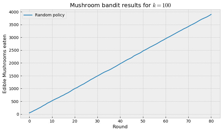
We first play the game with a random policy. The code for running an episode of the game is very simple:
# number of mushrooms eaten per round
K = 100

# instance of the game
mb = MushroomBandit(X, y)

# we initialize the agent by eating the first 50 mushrooms of the base
round_feedback = mb.eat_mushrooms(mb.get_not_eaten().head(50).index)

# and we get the number of rounds
n_rounds = int(mb.get_not_eaten().shape[0]/K) + 1

# list and to accumulate rewards
cum_rewards = 0
cum_rewards_list_random = []

# then, we play until no mushrooms are left
for round_id in tqdm(range(n_rounds)):

    # choosing random mushrooms
    to_eat = np.random.choice(mb.get_not_eaten().index, K)

    # eating
    feedback = mb.eat_mushrooms(to_eat)

    # saving cumulative rewards
    cum_rewards += feedback.sum()
    cum_rewards_list_random.append(cum_rewards)
At the end of game we inspect the number of edible mushrooms eaten during the course of the episode. The random policy fares as we would expect: a straight line, as it eats edible mushrooms at the same rate as poisonous ones (considering class imbalance).
We then proceed to replacing the random policy with a regular neural network and our bootstrapped neural network. The regular net is the same as a greedy method, as it only uses the expectation learned by the net to make decisions. The bootstrapped net emulates Thompson Sampling, as each head acts like a sample of a posterior distribution. Thus, we expect that the BNN explores efficiently and makes better decisions than the regular net. The plot below shows the results achieved:
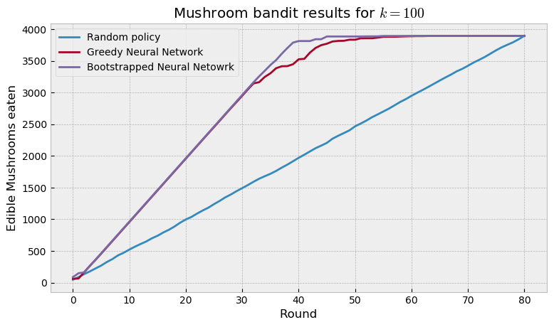
As we would expect, the boostrapped net finds all the edible mushrooms faster than the regular net, as it explores more efficiently. This technique provides a good bayesian approximation to neural networks, and can be used in a number of other settings. There’s great discussion about bayesian deep learning right now, particularly concerning the advantages of this approach compared to Monte Carlo dropout. I look forward to seeing the evolution of the field in the next years.
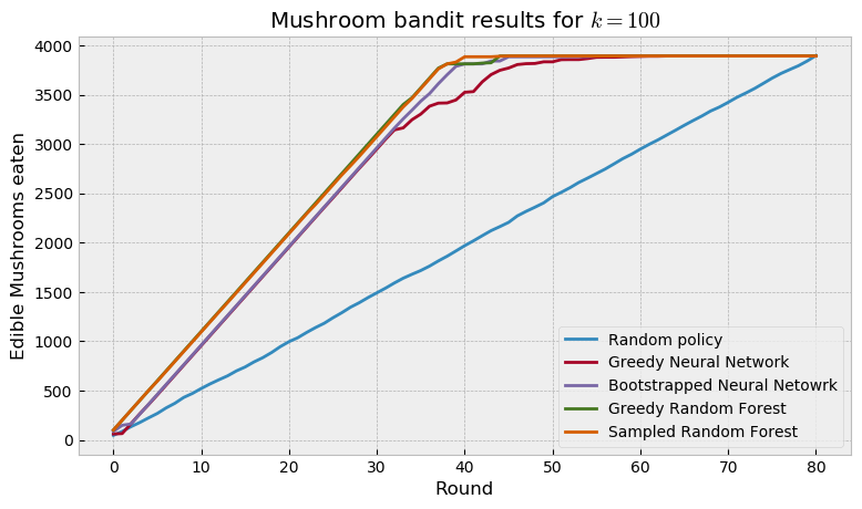
Finally, we run a regular (greedy) RF against our sampled RF. Interestingly, both RF models beat neural networks, with the sampled RF overcoming the greedy RF only at the very end of game. This is a very curious result, which teases us to test the models in other datasets. If you want to do that, remember that the code for this experiment is freely available at my GitHub page.
Conclusion
Even that the mushroom bandit was easily solved by the models, we can check that randomizing decisions offer improvements over greedy decisions. On the final plot the randomized models outperformed the greedy models, especially on the hardest mushrooms (the last ones to be eaten). In this particular case, Random Forest compared favourably against neural networks, and are trained and sampled in a fraction of the time.
In the future, we should try out other methods like UCB and $\epsilon$-greedy, and check if they will be outperformed by Thompson Sampling, as recent research suggests.