In this post, I’ll try out a new way to represent data and perform clustering: forest embeddings. A forest embedding is a way to represent a feature space using a random forest. Each data point $x_i$ is encoded as a vector $x_i = [e_0, e_1, …, e_k]$ where each element $e_i$ holds which leaf of tree $i$ in the forest $x_i$ ended up into. The encoding can be learned in a supervised or unsupervised manner:
Supervised: we train a forest to solve a regression or classification problem. Then, we use the trees structure to extract the embedding.
Unsupervised: each tree of the forest builds splits at random, without using a target variable.
There may be a number of benefits in using forest-based embeddings:
Distance calculations are ok when there are categorical variables: as we’re using leaf co-ocurrence as our similarity, we do not need to be concerned that distance is not defined for categorical variables.
For supervised embeddings, we automatically set optimal weights for each feature for clustering: if we want to cluster our data given a target variable, our embedding automatically selects the most relevant features.
We do not need to worry about scaling features: we do not need to worry about the scaling of the features, as we’re using decision trees.
In the next sections, we implement some simple models and test cases. You can find the complete code at my GitHub page.
Building the embeddings
So how do we build a forest embedding? It’s very simple. We start by choosing a model. In our case, we’ll choose any from RandomTreesEmbedding, RandomForestClassifier and ExtraTreesClassifier from sklearn. Let’s say we choose ExtraTreesClassifier. The first thing we do, is to fit the model to the data.
# choosing and fitting a model
model = ExtraTreesClassifier(n_estimators=100, min_samples_leaf=10)
model.fit(X, y)
As we’re using a supervised model, we’re going to learn a supervised embedding, that is, the embedding will weight the features according to what is most relevant to the target variable. Data points will be closer if they’re similar in the most relevant features. After model adjustment, we apply it to each sample in the dataset to check which leaf it was assigned to.
# let us apply to X
leaves = model.apply(X)
Then, we apply a sparse one-hot encoding to the leaves:
# applying a one-hot encoding scheme
M = OneHotEncoder().fit_transform(leaves)
At this point, we could use an efficient data structure such as a KD-Tree to query for the nearest neighbours of each point. To simplify, we use brute force and calculate all the pairwise co-ocurrences in the leaves using dot products:
# we perform M*M.transpose(), which is the same to
# computing all the pairwise co-ocurrences in the leaves
S = (M*M.transpose()).todense()

# lastly, we normalize and subtract from 1, to get dissimilarities
D = 1 - S/S.max()
Finally, we have a D matrix, which counts how many times two data points have not co-occurred in the tree leaves, normalized to the [0,1] interval. D is, in essence, a dissimilarity matrix.
The last step we perform aims to make the embedding easy to visualize. We feed our dissimilarity matrix D into the t-SNE algorithm, which produces a 2D plot of the embedding.
# computing 2D embedding with tsne, for visualization purposes
 embed = TSNE(metric='precomputed', perplexity=30).fit_transform(D)
In the next sections, we’ll run this pipeline for various toy problems, observing the differences between an unsupervised embedding (with RandomTreesEmbedding) and supervised embeddings (Ranfom Forests and Extremely Randomized Trees). We favor supervised methods, as we’re aiming to recover only the structure that matters to the problem, with respect to its target variable.
Two blobs, two dimensions
Let us start with a dataset of two blobs in two dimensions.
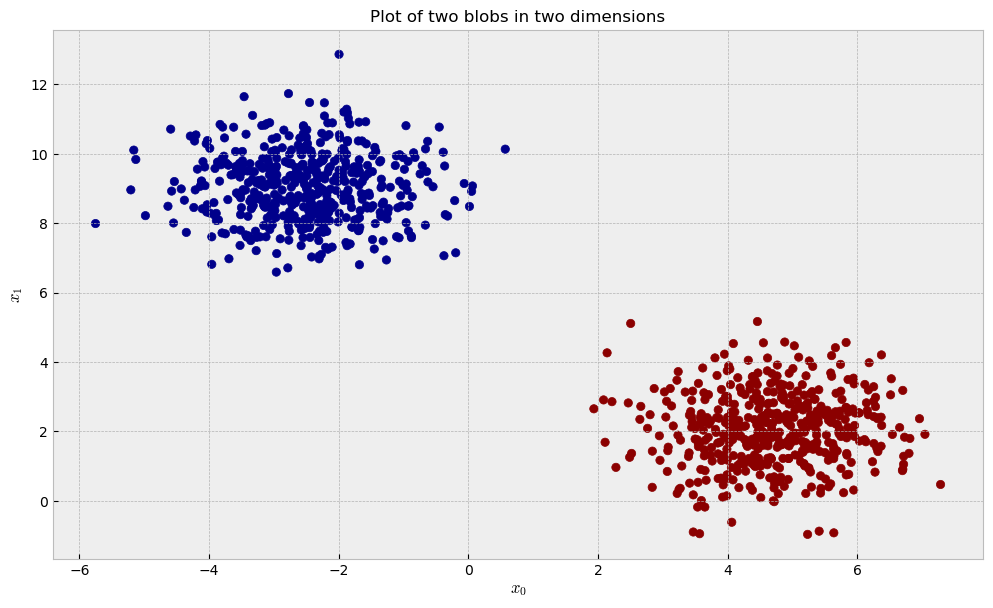
As the blobs are separated and there’s no noisy variables, we can expect that unsupervised and supervised methods can easily reconstruct the data’s structure thorugh our similarity pipeline. After we fit our three contestants (RandomTreesEmbedding, RandomForestClassifier and ExtraTreesClassifier) to the data, we can take a look at the similarities they learned and the plot below:
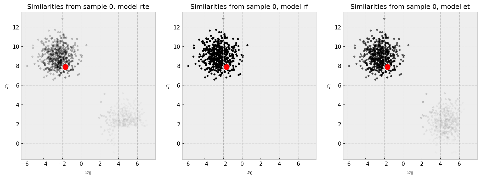
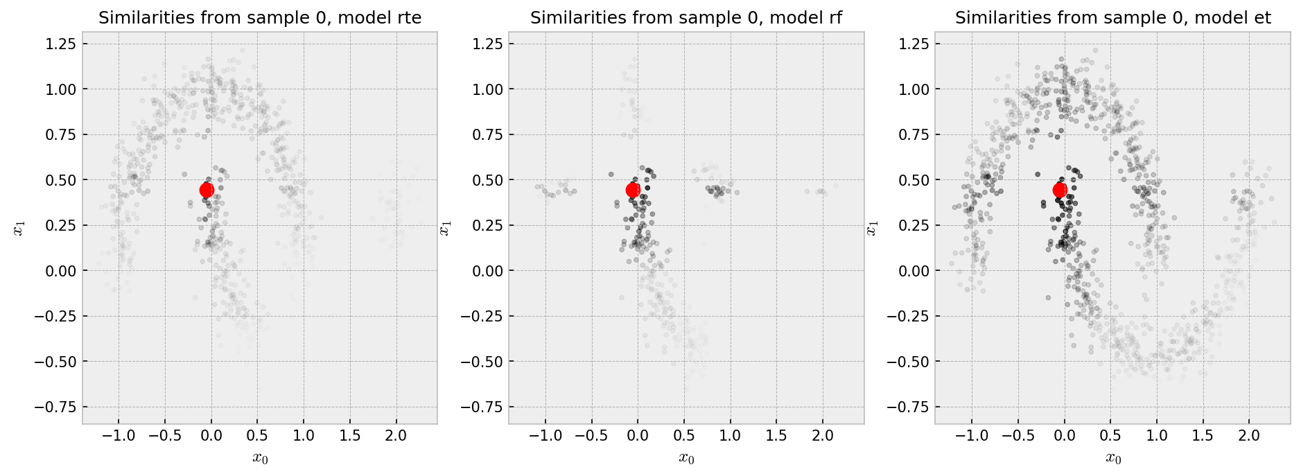
The red dot is our “pivot”, such that we show the similarity of all the points in the plot to the pivot in shades of gray, black being the most similar. Each plot shows the similarities produced by one of the three methods we chose to explore. Similarities by the RF are pretty much binary: points in the same cluster have 100% similarity to one another as opposed to points in different clusters which have zero similarity. ET and RTE seem to produce “softer” similarities, such that the pivot has at least some similarity with points in the other cluster.
Finally, let us check the t-SNE plot for our methods. In the upper-left corner, we have the actual data distribution, our ground-truth. The other plots show t-SNE reconstructions from the dissimilarity matrices produced by methods under trial.
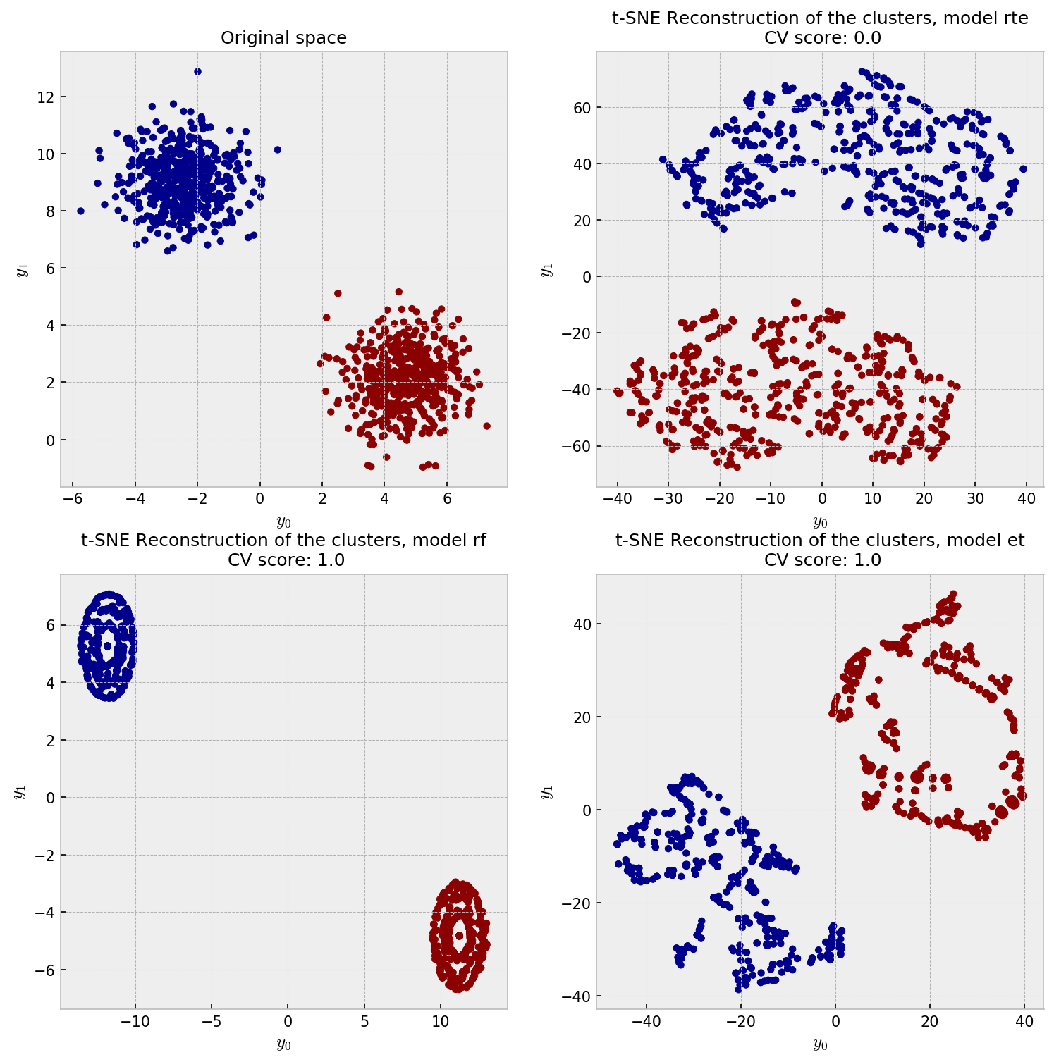
All the embeddings give a reasonable reconstruction of the data, except for some artifacts on the ET reconstruction. I’m not sure what exactly are the artifacts in the ET plot, but they may as well be the t-SNE “overfitting” the local structure, close to the artificial clusters shown in the gaussian noise example in here.
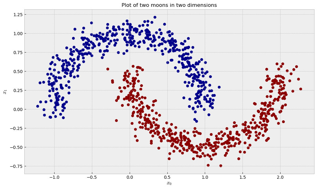
Two moons, two dimensions
Now, let us check a dataset of two moons in two dimensions, like the following:
The similarity plot shows some interesting features:
And the t-SNE plot shows some weird patterns for RF and good reconstruction for the other methods:
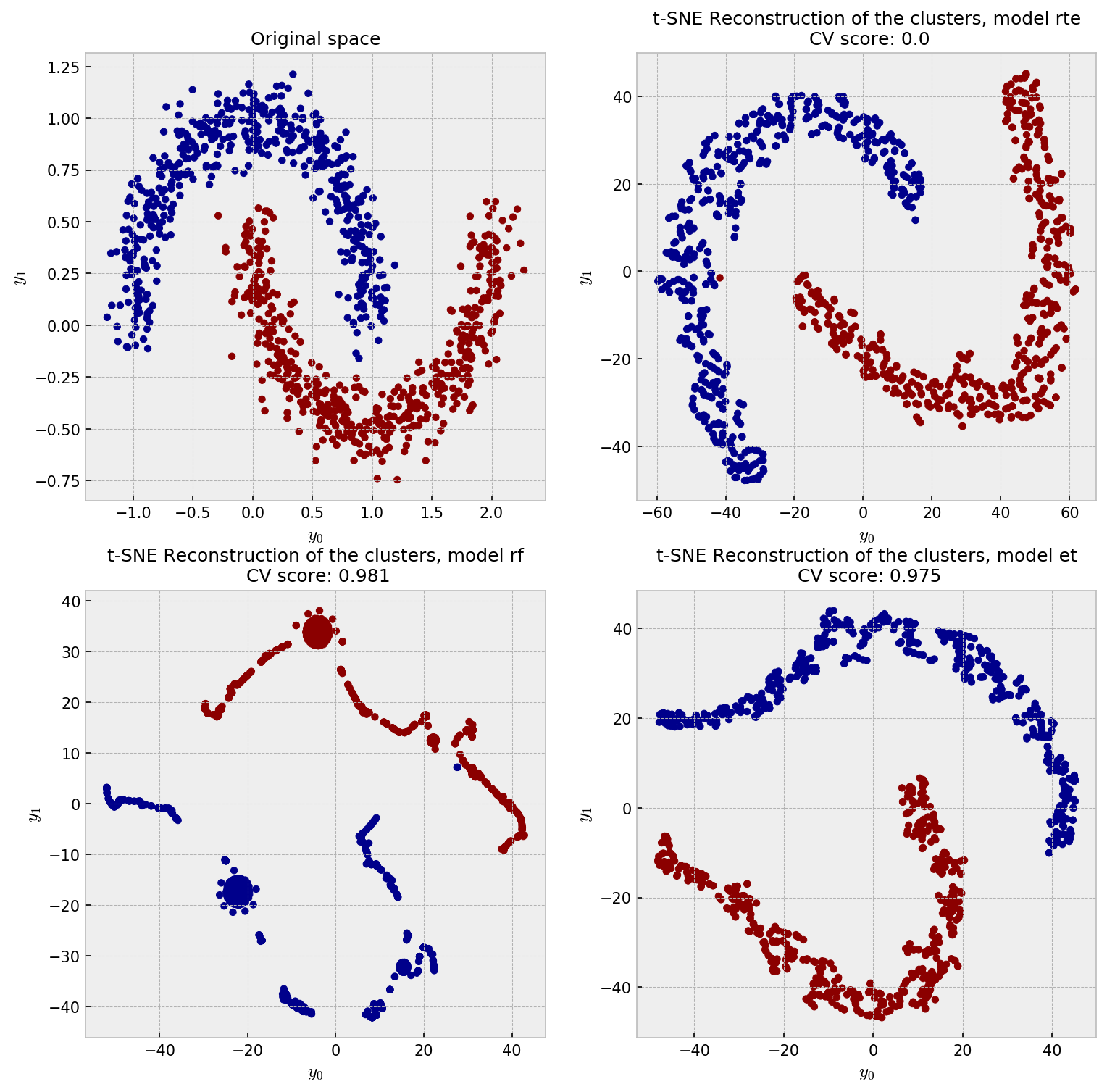
RTE perfectly reconstucts the moon pattern, while ET unwraps the moons and RF shows a pretty strange plot. I think the ball-like shapes in the RF plot may correspond to regions in the space in which the samples could be perfectly classified in just one split, like, say, all the points in $y_1 < -0.25$. All of these points would have 100% pairwise similarity to one another. As ET draws splits less greedily, similarities are softer and we see a space that has a more uniform distribution of points.
Four moons, where only two are relevant
Now, let us concatenate two datasets of moons, but we will only use the target variable of one of them, to simulate two irrelevant variables. The following plot shows the distribution for the four independent features of the dataset, $x_1$, $x_2$, $x_3$ and $x_4$. $x_1$ and $x_2$ are highly discriminative in terms of the target variable, while $x_3$ and $x_4$ are not. The following plot makes a good illustration:
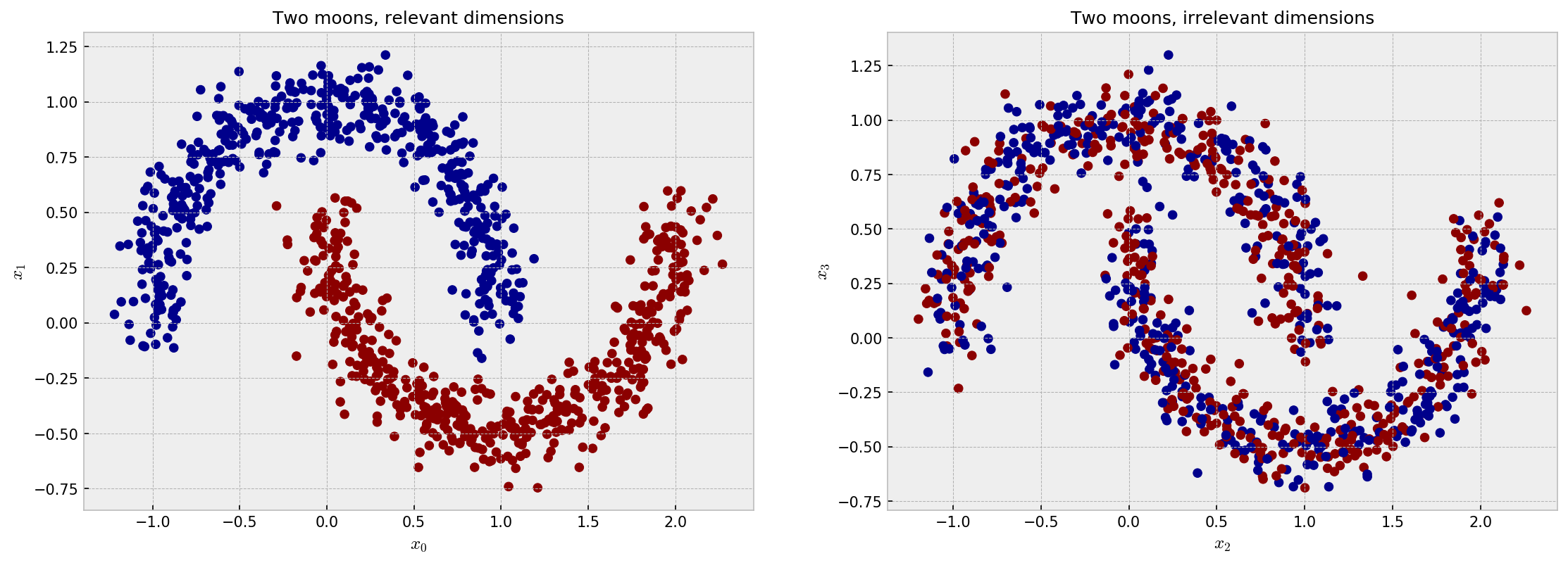
The ideal embedding should throw away the irrelevant variables and reconstruct the true clusters formed by $x_1$ and $x_2$. Intuition tells us the only the supervised models can do this. As it’s difficult to inspect similarities in 4D space, we jump directly to the t-SNE plot:
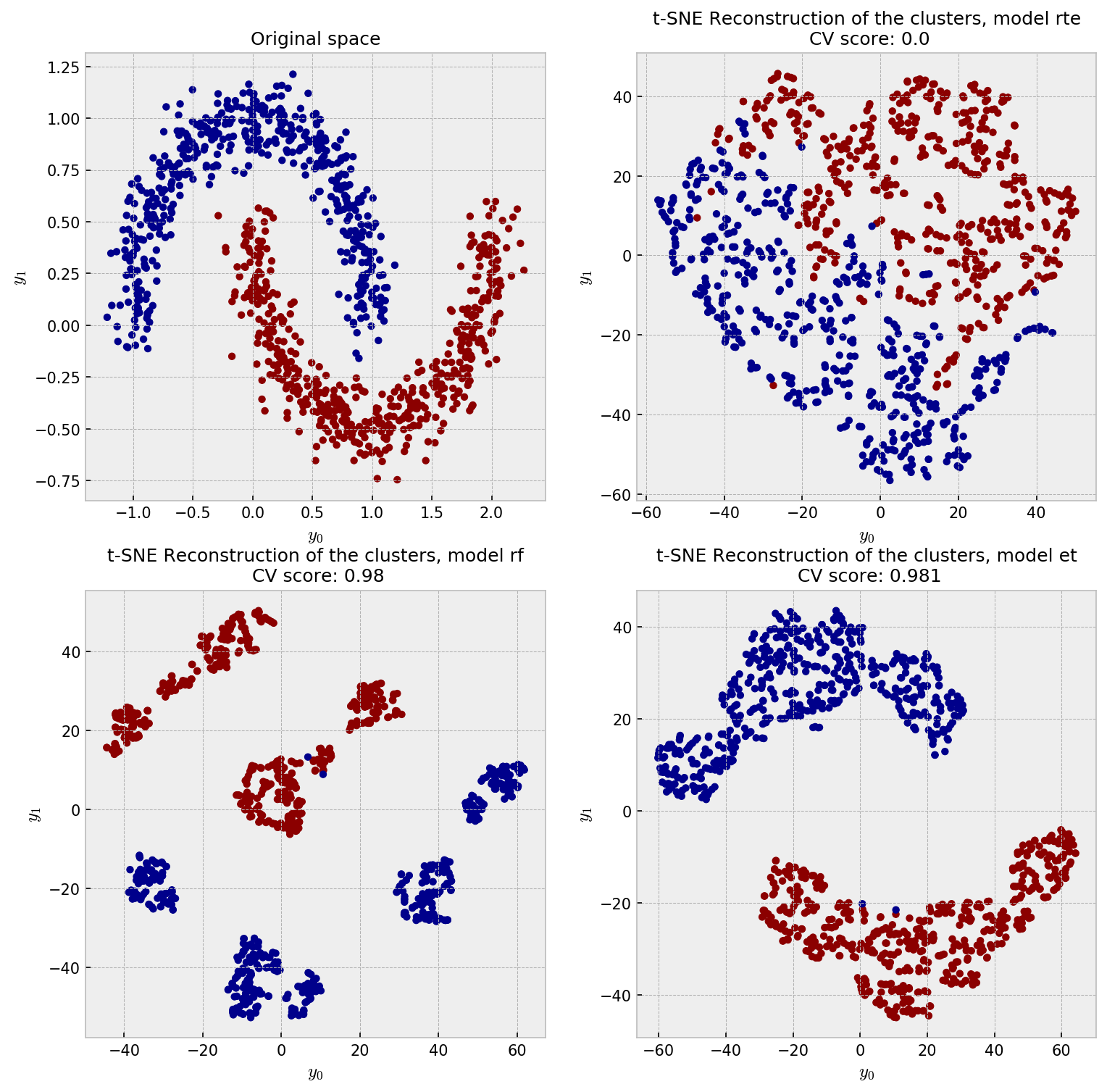
As expected, supervised models outperform the unsupervised model in this case. RTE suffers with the noisy dimensions and shows a meaningless embedding. RF, with its binary-like similarities, shows artificial clusters, although it shows good classification performance. ET wins this competition showing only two clusters and slightly outperforming RF in CV.
Real case: Boston housing dataset
Finally, let us now test our models out with a real dataset: the Boston Housing dataset, from the UCI repository. Here’s a snippet of it:
| CRIM | ZN | INDUS | CHAS | NOX | RM | AGE | DIS | RAD | TAX | PTRATIO | B | LSTAT |
|---|---|---|---|---|---|---|---|---|---|---|---|---|
| 0.00632 | 18.0 | 2.31 | 0.0 | 0.538 | 6.575 | 65.2 | 4.0900 | 1.0 | 296.0 | 15.3 | 396.90 | 4.98 |
| 0.02731 | 0.0 | 7.07 | 0.0 | 0.469 | 6.421 | 78.9 | 4.9671 | 2.0 | 242.0 | 17.8 | 396.90 | 9.14 |
| 0.02729 | 0.0 | 7.07 | 0.0 | 0.469 | 7.185 | 61.1 | 4.9671 | 2.0 | 242.0 | 17.8 | 392.83 | 4.03 |
| 0.03237 | 0.0 | 2.18 | 0.0 | 0.458 | 6.998 | 45.8 | 6.0622 | 3.0 | 222.0 | 18.7 | 394.63 | 2.94 |
| 0.06905 | 0.0 | 2.18 | 0.0 | 0.458 | 7.147 | 54.2 | 6.0622 | 3.0 | 222.0 | 18.7 | 396.90 | 5.33 |
This is a regression problem where the two most relevant variables are RM and LSTAT, accounting together for over 90% of total importance. We plot the distribution of these two variables as our reference plot for our forest embeddings. The color of each point indicates the value of the target variable, where yellow is higher. Let us check the t-SNE plot for our reconstruction methodologies.
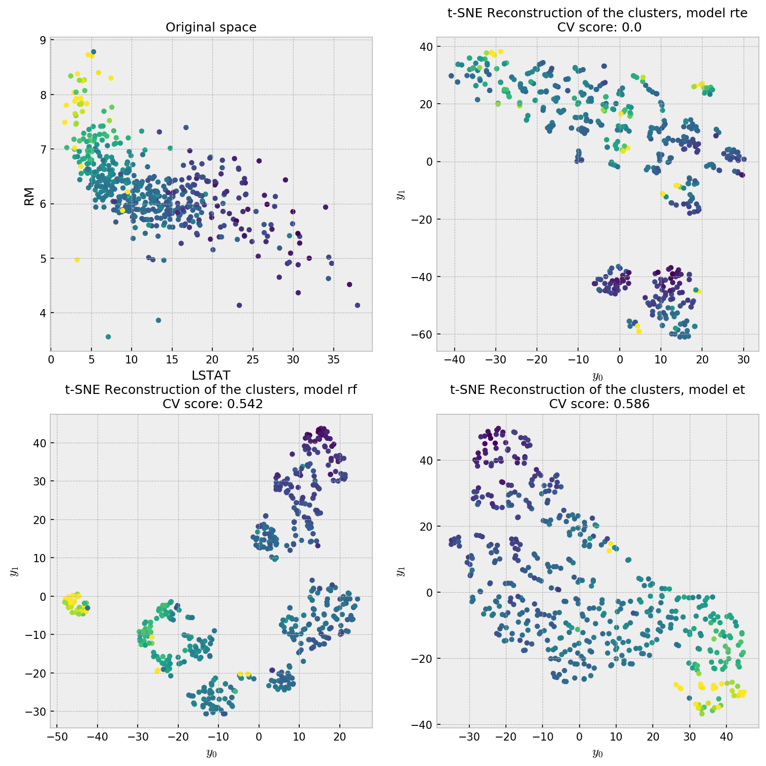
The first plot, showing the distribution of the most important variables, shows a pretty nice structure which can help us interpret the results. RTE is interested in reconstructing the data’s distribution, so it does not try to put points closer with respect to their value in the target variable. The supervised methods do a better job in producing a uniform scatterplot with respect to the target variable. Considering the two most important variables (90% gain) plot, ET is the closest reconstruction, while RF seems to have created artificial clusters. This is further evidence that ET produces embeddings that are more faithful to the original data distribution.
Conclusion
In this tutorial, we compared three different methods for creating forest-based embeddings of data. The unsupervised method Random Trees Embedding (RTE) showed nice reconstruction results in the first two cases, where no irrelevant variables were present. When we added noise to the problem, supervised methods could move it aside and reasonably reconstruct the real clusters that correlate with the target variable. Despite good CV performance, Random Forest embeddings showed instability, as similarities are a bit binary-like. However, Extremely Randomized Trees provided more stable similarity measures, showing reconstructions closer to the reality. We conclude that ET is the way to go for reconstructing supervised forest-based embeddings in the future.