In this post, we’ll build on the Multi-Armed Bandit problem by relaxing the assumption that the reward distributions are stationary. Non-stationary reward distributions change over time, and thus our algorithms have to adapt to them. There’s simple way to solve this: adding buffers. Let us try to do it to an $\epsilon$-greedy policy and Thompson Sampling. Please, feel free to get the full code in my GitHub page.
Problem statement
Let us define some test cases where the reward distributions can change over time and implement them. In this Notebook, we assume that the rewards $r_k$ are binary, and distributed according to a Bernoulli random variable $r_k \sim Bernoulli(\theta_k)$, where $\theta_k$ is our reward parameter, the expected reward at each round.
Reward parameters change according to some distribution every $K$ rounds: let us define each of our reward parameters $\theta_k$ as a random variable, say, $\theta_k \sim \mathcal{U}(0,1)$, and sample a new reward parameter vector for our bandits $\theta$ every $K$ rounds. The algoritms must adapt to the new conditions, which suddenly change.
Reward parameters change linearly over time: in this case, we set two reward parameter vectors, $\theta_0$ and $\theta_1$, and linearly change the actual reward vector from $\theta_0$ and $\theta_1$ during $K$ rounds. So, if $n$ is the number of rounds that we have played so far, our reward vector is $\theta = (1 - \frac{n}{K}) \cdot{} \theta_0 + \frac{n}{K} \cdot{} \theta_1$.
We can easily implement a class to play this bandit game in Python:
# now implementing non stationary MABs on top
class NonStationaryMAB:

    # initialization
    def __init__(self, bandit_probs_1, K, bandit_probs_dist, mode='dist', bandit_probs_2=None):

        # storing parameters
        self.K = K
        self.bandit_probs_dist = bandit_probs_dist
        self.mode = mode
        self.bandit_probs_1 = np.array(bandit_probs_1)
        self.bandit_probs_2 = np.array(bandit_probs_2)

        # initializing actual bandit probabilities
        self.bandit_probs = self.bandit_probs_1

    # function for drawing arms
    def draw(self, k, n):

        # selecting mode
        if self.mode == 'dist':

            # need to update reward parameters?
            if ((n % self.K) == 0) & (n != 0):
                self.bandit_probs = self.bandit_probs_dist.rvs(len(self.bandit_probs))

        # selecting mode
        elif self.mode == 'linear':

            # updating parameters
            if (n <= self.K) & (n >= 0):
                self.bandit_probs = (1 - n/self.K)*self.bandit_probs_1 + n/self.K*self.bandit_probs_2

        # if no known mode is selected, raise error
        else:
            raise ValueError()

        # guaranteeing that values are in the 0, 1 range
        self.bandit_probs = np.clip(self.bandit_probs, 0, 1)

        # returning a reward for the current arm
        return np.random.binomial(1, self.bandit_probs[k]), np.max(self.bandit_probs) - self.bandit_probs[k]
Let us simulate the first challenge with a random policy. In the following plot $K = 100$ and new reward parameters $\theta_k$ are drawn from a uniform distribution $\theta_k \sim \mathcal{U}(0, 1)$.
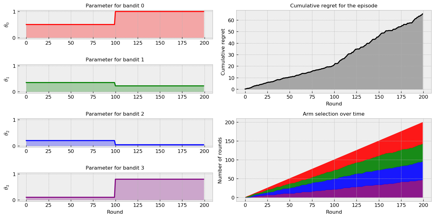
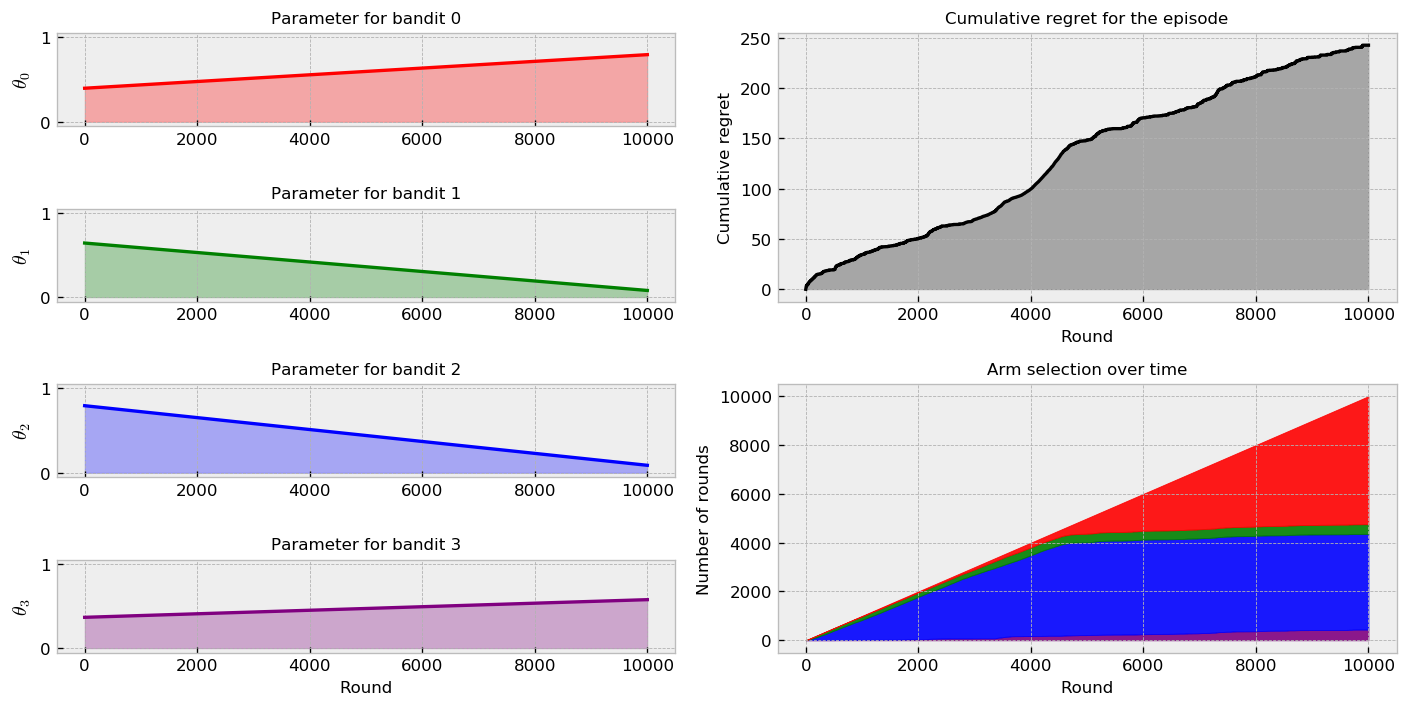
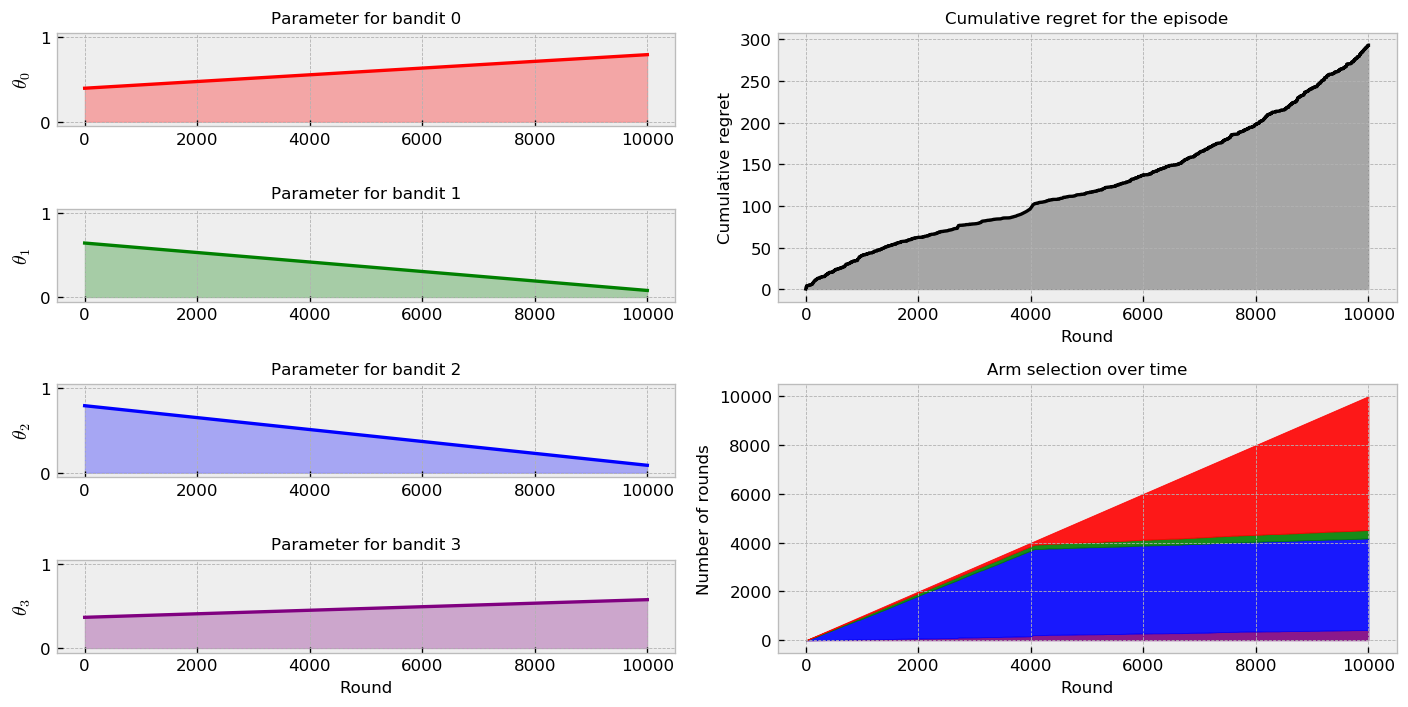
We can inspect six different plots in the figure. At the left-hand side, the plots show true expected reward over time for each bandit. In this case, we observe step functions, as the change in parameters is sudden. At the upper right-hand side, we can inspect the cumulative regret $\theta_{best} - \theta_k$ plot for the policy. The flatter is the regret plot, the better. Finally, at the lower right-hand side, we can inspect the cumulative arm selection plot, showing hoy many times we selected each arm during the episode. As we’re using a random policy, the selection proportion is balanced and does not change with the change in true bandit parameters.
Now, let us simulate the second challenge. We set $K = 200$ so that the transition from $\theta_0$ to $\theta_1$ ends at the same time as the episode.
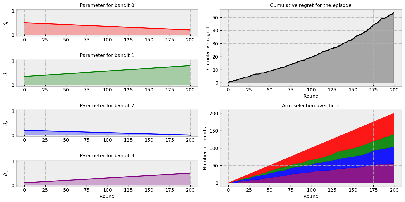
In this case, the change in parameters is not sudden like in the previous one. Instead, we observe a linear and continuous change. As the policy is random, arm selection rates are like the previous case. The regret plot interpretation is also the same. Let us implement our policies and check if they shift their selection as one arm becomes better than the others.
Policies
Let us implement a $\epsilon$-greedy policy along with Thompson Sampling. For both policies, we implement a buffer, which is the size of the game history we want the policies to remember to make their decisions. The smaller the buffer is, the algorithm explores more and can better adapt to the changes in the parameters. However, it may also waste useful opportunity to exploit the system.
There is a trade-off between these two issues in deciding the size of the buffer. For people doing data science in industry, the size of the buffer may be defined by business expert knowledge (the number of days that the market takes to react to a pricing decision, for instance).
We can implement the policies with just a few changes from the ones in the first Thompson Sampling tutorial:
# e-greedy policy
class eGreedyPolicy:

    # initializing
    def __init__(self, epsilon, buffer_size):

        # saving parameters
        self.epsilon = epsilon
        self.buffer_size = buffer_size

    # choice of bandit
    def choose_bandit(self, k_array, reward_array, n_bandits):

        # number of plays
        n_plays = int(k_array.sum())

        # limiting the size of the buffer
        reward_array = reward_array[:,:n_plays][:,-self.buffer_size:]
        k_array = k_array[:,:n_plays][:,-self.buffer_size:]

        # sucesses and failures
        success_count = reward_array.sum(axis=1)
        total_count = k_array.sum(axis=1)

        # ratio of sucesses vs total
        success_ratio = success_count/total_count

        # choosing best greedy action or random depending with epsilon probability
        if np.random.random() < self.epsilon:

            # returning random action, excluding best
            return np.random.choice(np.delete(list(range(N_BANDITS)), np.argmax(success_ratio)))

        # else return best
        else:

            # returning best greedy action
            return np.argmax(success_ratio)

 # thompson sampling
class TSPolicy:

    # initializing
    def __init__(self, buffer_size):

        # nothing to do here
        self.buffer_size = buffer_size

    # choice of bandit
    def choose_bandit(self, k_array, reward_array, n_bandits):

        # number of plays
        n_plays = int(k_array.sum())

        # limiting the size of the buffer
        reward_array = reward_array[:,:n_plays][:,-self.buffer_size:]
        k_array = k_array[:,:n_plays][:,-self.buffer_size:]

        # list of samples, for each bandit
        samples_list = []

        # sucesses and failures
        success_count = reward_array.sum(axis=1)
        failure_count = k_array.sum(axis=1) - success_count

        # drawing a sample from each bandit distribution
        samples_list = [np.random.beta(1 + success_count[bandit_id], 1 + failure_count[bandit_id]) for bandit_id in range(n_bandits)]

        # returning bandit with best sample
        return np.argmax(samples_list)
Challenge 1
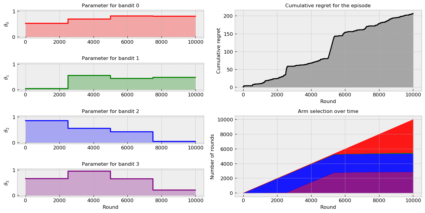
Let us measure how well our methods fare in the first challenge. Let us start with the Thompson Sampling plot:
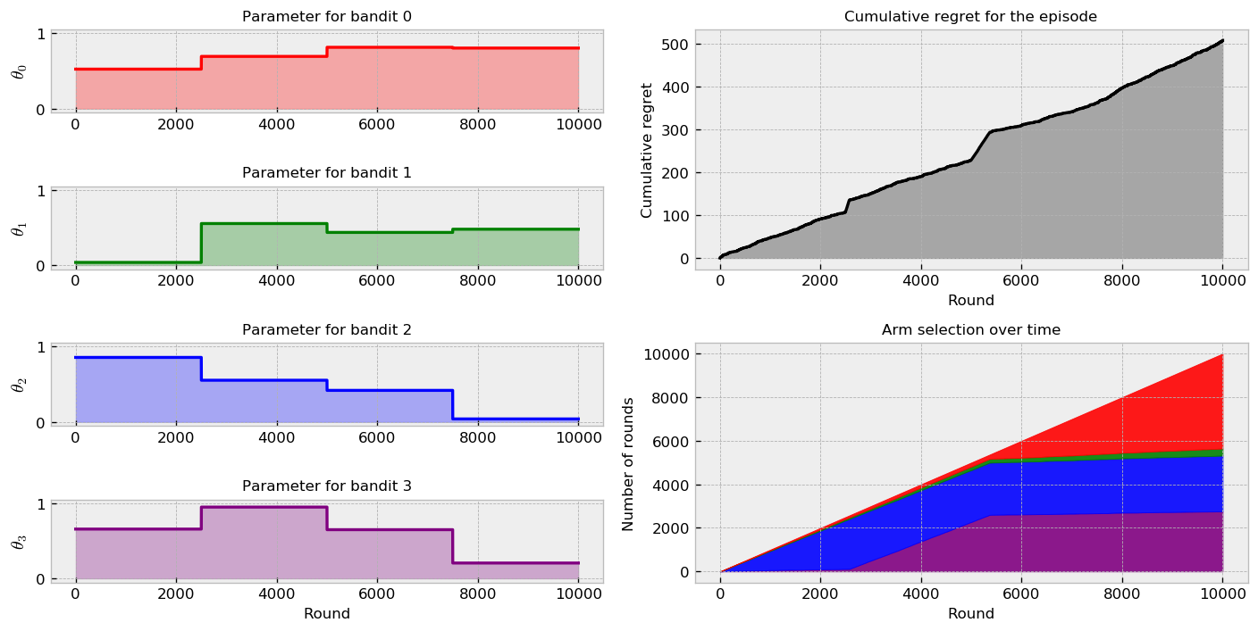
Now, we show results for the $\epsilon$-greedy policy:
Let us compare the methodologies on several simulations as well. The following regret plot compares the algorithms:
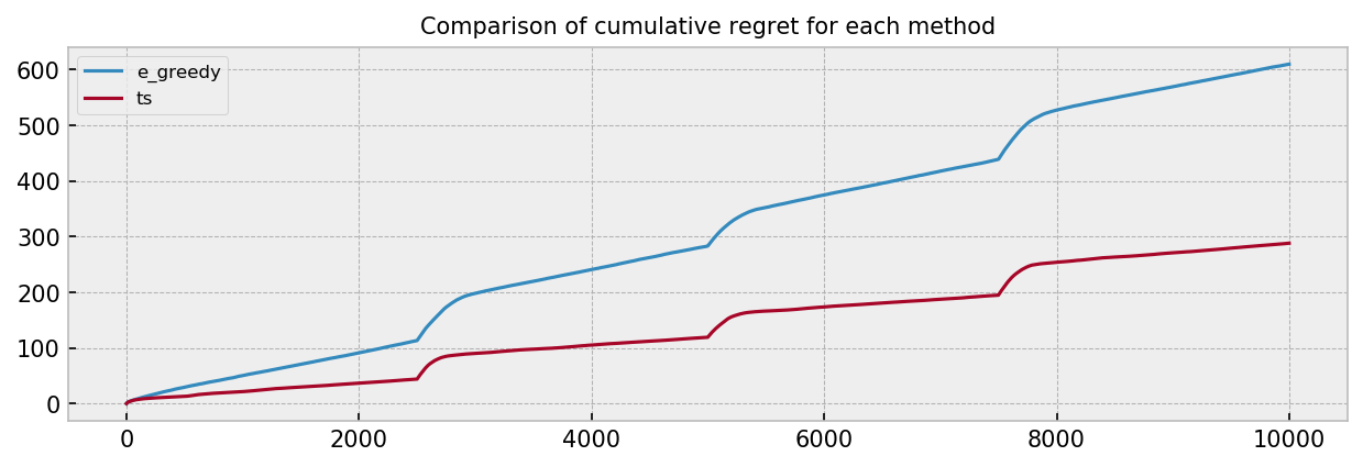
The results show that Thompson Sampling compares favourably against the $\epsilon$-greedy policy. The combined visualizations show much better performance of TS in the first game. We can see that TS quickly adapted to changing parameters, maintaining a good dose of exploration. Seems like the $\epsilon$-greedy policy over-explored in the entire game, so tuning the $\epsilon$ parameters could be an improvement here. The comparison plot over many simulations also shows great improvement by using TS, with smaller final cumulative regret. We can also see some bumps in the plot at the times of sudden parameter change, showing how much time the algorithms take to adapt to the new conditions.
Challenge 2
Let us measure how well our methods fare in the second challenge. Let us start with TS:
Moving to $\epsilon$-greedy:
Anf finally to the comparison plot over many simulations:
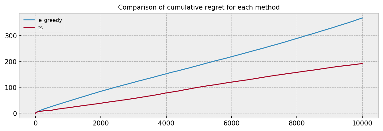
The results resemble the ones obtained in the first challenge. Again, $\epsilon$-greedy seems to be over-exploring. The combined visualizations show that TS is much quicker to start playing the best arm. The comparison plot shows a substantial improvement by using TS as well. We do not see the “regret bumps” as before, because our parameters now vary linearly over the course of the episode.
Buffer size analysis
Up until now, we ran all our analyses with a buffer size of 500. Can we do better? Let us evaluate how the buffer size influences the adaptability of the Thompson Sampling policy. We show a regret comparison plot for buffer sizes 50, 100, 250, 500, 1000, 2500 and 5000 over many simulations, for the first challenge. Each line represents the Thompson Sampling policy with a different buffer size.

The green line shows regret for TS with buffer size 500 and seems like the best option overall. We can see that policies with larger buffers fare really well in the first quarter of the simulation, but their regret explodes when the first parameter transition kicks in. The ideal policy would have a very large buffer just before the transition and a very small buffer just after the transition. An interesting problem is to devise an adaptive policy that could correct its buffer size. We leave this problem for the future.
Conclusion
In this Notebook, we studied non-stationary bandits, which the distribution of true expected rewards $\theta$ changes over time. We presented two scenarios: (a) $\theta$ changes suddenly and (b) $\theta$ changes slowly and linearly. In both cases, Thompson Sampling compared favourably to an $\epsilon$-greedy policy. Using a buffer was beneficial such that TS explored more and could quickly adapt to changes in the bandits true parameters. In our final experiment, we tested different buffer sizes and observed TS cumulative regret over many simulations. Small buffer sizes perform little exploitation, with cumulative regret being close to linear. On the other hand, large buffer sizes show great regret results only until the first parameter change, when they make TS very slow to adapt to the new conditions. In our setting, we could find a good tradeoff. In business situations, a subject matter expert could advise on buffer sizes, giving insight on how much the system can change over time.