Let us experiment with different techniques for approximate bayesian inference aiming at using Thomspon Sampling to solve bandit problems, drawing inspiration from the paper “A Tutorial on Thompson Sampling”, mainly from the ideas on section 5. Let us test the algorithms on a simple bandit with gaussian rewards, such that we can compare our approximate inference techniques with the exact solution, obatined through a conjugate prior. I’ll implement and compare the following approximation techniques:
- Exact inference, where we use a conjugate prior to analytically update the posterior
- MCMC sampling, where we approximate the posterior by an empirical distribution obtained through the Metropolis-Hastings algorithm
- Variational Inference, where we approximate the posterior by trying to match it to an arbitrarily chosen variational distribution
- Bootstrapping, where we approximate the posterior by an empirical distribution obtained through bootstrap samples of the data
The Gaussian Bandit
Let us change up a bit from previous posts and experiment with bandits that produce continuous-valued rewards. We’ll choose the Gaussian distribution as ground-truth for generating rewards. Thus, each bandit $k$ can be modeled as a random variable $Y_k \sim \mathcal{N}(\mu_k, \sigma_k^2)$. The code that implements this bandit game is simple:
# class for our row of bandits
class GaussianMAB:

    # initialization
    def __init__(self, mu, sigma):

        # storing mean and standard deviation vectors
        self.mu = mu
        self.sigma = sigma

    # function that helps us draw from the bandits
    def draw(self, k):

        # we return the reward and the regret of the action
        return np.random.normal(self.mu[k], self.sigma[k]), np.max(self.mu) - self.mu[k]
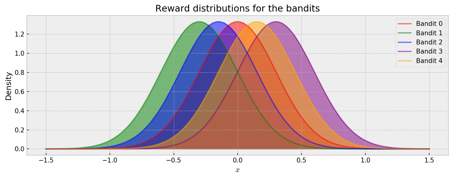
The distribution of rewards for each bandit is shown below. At each round, the player chooses one bandit $k$ and receives a reward according to one of the distributions $Y_k \sim \mathcal{N}(\mu_k, \sigma_k^2)$. As we want to focus on approximate inference, the problem is simplified so all the reward distributions have the same stardard deviation. I’ll explore reward distributions of different risks in the future.
Let us check the usual visualization of rewards over time. In the animation, each draw is represented by a dot with size proportional to the reward. Each horizontal line represents one of five bandits.
Cool. By visual inspection, it becomes clear that Bandits 1 and 2 are not very promising, while conclusions about the others are not that immediate. So how can we model the expected rewards for each bandit as the game progresses? This is the central question in this post. Let us start with a natural baseline for comparison: exact inference.
Exact inference
Our goal in this tutorial is to estimate the probability distribution of the mean (or expected) rewards $\mu_k$ for each bandit $k$ given some observations $x_k$. We can use Bayes formula to do that:
\[\large P(\mu_k\ \vert\ x_k) = \frac{P(x_k\ \vert\ \mu_k) \cdot{} P(\mu_k)}{P(x_k)}\]If you need a refresher, $P(\mu_k\ \vert\ x_k)$ is the posterior distribution and our quantity of interest, $P(x_k\ \vert\ \mu_k)$ is the likelihood, $P(\mu_k)$ is the prior and $P(x_k)$ is the model evidence. The first two quantities are easy to compute, as they depend on the parameters we want to estimate. The last quantity, the evidence $P(x_k)$ is harder, as it measures the probability of data given the model, that is, the likelihood of the data over all possible parameter choices:
\[\large P(x_k) = \int_{\mu_k} P(x_k\ \vert\ \mu_k) \, \mathrm{d}\mu_k\]In other settings we won’t solve Bayes formula because calculating this integral is intractable, especially when we have more parameters. However, in our simple case, we can get the posterior analytically through a property called conjugacy. When the prior and posterior distributions are of the same family for a given likelihood, they’re called conjugate distributions, and the prior is called a conjugate prior for the likelihood function. When the data is Gaussian distributed, the prior and posterior for the mean of the data generating process are also Gaussian. To make things easier, we assume we know the standard deviation of the likelihood beforehand. We can perform this same inference with an unknown $\sigma$, but I’ll leave it to the future. We just need to calculate, for each bandit $k$, and given prior paramaters $\mu^0_k$ and $\sigma^0_k$, the posterior after seeing $n$ observations $\mu^n_k$:
\[\large \mu^n_k \sim \mathcal{N}\Bigg(\frac{1}{\frac{1}{(\sigma^0_k)^2} + \frac{n}{({\sigma_{true_k}})^2}}\Bigg(\frac{\mu^0_k}{(\sigma^0_k)^2} + \frac{\sum_{i=1}^n x_i}{({\sigma_{true_k}})^2}\Bigg),\Bigg(\frac{1}{(\sigma^0_k)^2} + \frac{n}{({\sigma_{true_k}})^2}\Bigg)^{-1}\Bigg)\]Where $\large \sigma_{true_k}$ is the known standard deviation of our Gaussian likelihood, for each bandit $k$. We can easily implement this with a class in Python:
# class for exact gaussian inference
class ExactGaussianInference:

    # initializing with prior paramters
    def __init__(self, prior_mu, prior_sigma, likelihood_sigma):

        # storing
        self.prior_mu = prior_mu
        self.prior_sigma = prior_sigma
        self.post_mu = prior_mu
        self.post_sigma = prior_sigma
        self.likelihood_sigma = likelihood_sigma

    # fitting the posterior for the mean
    def get_posterior(self, obs):

        # checking if there is any observation before proceeding
        if len(obs) > 0:

            # calculating needed statistics for the observations
            obs_mu = np.mean(obs)
            obs_sum = np.sum(obs)
            obs_n = len(obs)

            # updating posterior mean
            self.post_mu = (1/(1/self.prior_sigma**2 + obs_n/self.likelihood_sigma**2) *
                            (self.prior_mu/self.prior_sigma**2 + obs_sum/self.likelihood_sigma**2))

            # updating posterior sigma
            self.post_sigma = (1/self.prior_sigma**2 + obs_n/self.likelihood_sigma**2)**(-1)

        # return posterior
        return norm_dist(self.post_mu, np.sqrt(self.post_sigma))
The following animation illustrates how our exact posterior inference algorithm works. It shows 100 draws from a $\mathcal{N}(0.2, 1.0)$ distribution, and the exact posterior distribution over its expected value.
The animation shows the exact posterior distribution (blue) given incremental data (red). We can see that exact inference is working as we would expect: the posterior distribution concentrates with more data, also getting closer to the true mean. The prior can act as a form of regularization here: if the prior is more concentrated, it is harder to move away from it. I invite you to try the code out to check that. The algorithm is very efficient: 100 calculations took 0.10 seconds in this experiment.
Even if we actually can calculate the posterior analytically in this case, most of the times it will not be possible, as we discussed previously. That’s where approximate inference comes into play. Let us apply it to the same problem and compare the results to exact inference.
MCMC Sampling
Let us now imagine that calculating the model evidence $P(x_k)$ is intractable and we cannot solve our inference problem analytically. In this case, we have to use approximate inference techniques. The first we’re going to try is Markov chain Monte Carlo sampling. This class of algorithms helps us to approximate posterior distributions by (roughly) making a random walk process gravitate around the maximum of the product of likelihood and prior density functions. Specifically, let us try to use the Metropolis-Hastings algorithm. I will first show how to implement it from scratch.
Metropolis-Hastings from scratch
It’s not very hard to implement the algorithm from scratch. For a more detailed tutorial, follow this excellent post which helped me a lot to understand what is going on under the hood.
Remember that we want to estimate the probability distribution of the mean $\mu_k$ for each bandit $k$ given some observations $x_k$. We can use Bayes formula do estimate that:
\[\large P(\mu_k\ \vert\ x_k) = \frac{P(x_k\ \vert\ \mu_k) \cdot{} P(\mu_k)}{P(x_k)}\]Calculating the product between the likelihood and prior $P(x_k\ \vert\ \mu_k) \cdot{} P(\mu_k)$ is easy. The problem lies in calculating the evidence $P(x_k)$, as it may become a very difficult integral (even if in our case is still tractable):
\[\large P(x_k) = \int_\mu P(x_k\ \vert\ \mu_k) \, \mathrm{d}\mu_k\]The Metropolis-Hastings algorithm bypasses this problem by only needing the prior and likelihood product. It starts by choosing a initial sampling point $\mu^t$ and defining a proposal distribution, which is generally a normal centered at zero $\mathcal{N}(0, \sigma_p^2)$. Then, it progresses as following:
- Initialize a list of samples
mu_listwith a single point $\mu^t$ and proposal distribution $\mathcal{N}(0, \sigma_p^2)$ - Propose a new sample $\mu^{t+1}$ using the proposal distribution $\mu^{t+1} = \mu^t + \mathcal{N}(0, \sigma_p^2)$
- Calculate the prior and likelihood product for the current sample $f(\mu^t) = P(x_k\ \vert\ \mu^t) \cdot{} P(\mu^t)$ and proposed sample $f(\mu^{t+1}) = P(x_k\ \vert\ \mu^{t+1}) \cdot{} P(\mu^{t+1})$
- Calculate the acceptance ratio $\alpha = f(\mu^{t+1})/f(\mu^t)$
- With probability $\alpha$, accept the proposed sample and add it to the list of samples
mu_list. If not accepted, add the current sample tomu_list, as we will propose a new sample from it again - Go back to (2) until a satisfactory number of samples is collected
It was proved that by accepting samples according to the acceptance ratio $\alpha$ our mu_list will contain samples that approximate the true posterior distribution. Thus, if we sample for long enough, we will have a reasonable approximation. The magic is that
such that the likelihood and prior product is sufficient to be proportional to the true posterior for us to get samples from it. We can easily implement this algorithm in Python:
# class for exact gaussian inference
class MetropolisHastingsGaussianInference:

    # initializing with prior paramters
    def __init__(self, prior_mu, prior_sigma, likelihood_sigma, proposal_width):

        # storing
        self.prior_mu = prior_mu
        self.prior_sigma = prior_sigma
        self.likelihood_sigma = likelihood_sigma
        self.proposal_width = proposal_width

    # fitting the posterior for the mean
    def get_posterior(self, obs, n_samples, burnin, thin):

        # checking if there is any observation before proceeding
        if len(obs) > 0:

            # our prior distribution and pdf for the observations
            prior_dist = norm_dist(self.prior_mu, self.prior_sigma)

            # our proposal distribution
            proposal_dist = norm_dist(0.0, self.proposal_width)

            # our list of samples
            mu_list = []

            # our initial guess, it will be the mean of the prior
            current_sample = self.prior_mu

            # loop for our number of desired samples
            for i in range(n_samples):

                # adding to the list of samples
                mu_list.append(current_sample)

                # our likelihood distribution for the current sample
                likelihood_dist_current = norm_dist(current_sample, self.likelihood_sigma)
                likelihood_pdf_current = likelihood_dist_current.logpdf(obs).sum()

                # our prior result for current sample
                prior_pdf_current =  prior_dist.logpdf(current_sample).sum()

                # the likelihood and prior product for current sample
                product_current = likelihood_pdf_current + prior_pdf_current

                # getting the proposed sample
                proposed_sample = current_sample + proposal_dist.rvs(1)[0]

                # our likelihood distribution for the proposed sample
                likelihood_dist_proposed = norm_dist(proposed_sample, self.likelihood_sigma)
                likelihood_pdf_proposed = likelihood_dist_proposed.logpdf(obs).sum()

                # our prior result for proposed sample
                prior_pdf_proposed =  prior_dist.logpdf(proposed_sample).sum()

                # the likelihood and prior product for proposed sample
                product_proposed = likelihood_pdf_proposed + prior_pdf_proposed

                # acceptance rate
                acceptance_rate = np.exp(product_proposed - product_current)

                # deciding if we accept proposed sample: if accepted, update current
                if np.random.uniform() < acceptance_rate:
                    current_sample = proposed_sample

            # return posterior density via samples
            return np.array(mu_list)[burnin::thin]

        else:

            # return samples from the prior
            return norm_dist(self.prior_mu, self.prior_sigma).rvs(int((n_samples - burnin)/thin))
The burnin argument sets how many of the initial samples will be discarded so we don’t calculate the posterior on samples taken when the algorithm was still on its ascent to the top of the unnormalized posterior density. Thinning, controlled by the thin argument, tells the algorithm to discard every $k$-th sample after burn-in, to reduce autocorrelation among samples. Let us visualize the algorithm working like we did in the exact inference case.
In the plot, we compare the exact posterior (blue), to the Metropolis-Hastings empirical approximation (purple). It works well, being very close to the exact posterior. But it is very slow, taking 185 seconds to calculate the posteriors to all of the 100 draws in my experiment. In order to improve that, let us try a better implementation.
Metropolis-Hastings with edward
Let us now use edward, a fairly recent Python library which connects tensorflow with probabilistic models. It supports the Metropolis-Hastings algorithm, which we will implement below:
# class for exact gaussian inference
class EdMetropolisHastingsGaussianInference:

    # initializing with prior paramters
    def __init__(self, prior_mu, prior_sigma, likelihood_sigma, proposal_width):

        # storing
        self.prior_mu = prior_mu
        self.prior_sigma = prior_sigma
        self.likelihood_sigma = likelihood_sigma
        self.proposal_width = proposal_width

    # fitting the posterior for the mean
    def get_posterior(self, obs, n_samples, burnin, thin):

        # checking if there is any observation before proceeding
        if len(obs) > 0:

            # making the computation graph variables self-contained and reusable
            with tf.variable_scope('mcmc_model', reuse=tf.AUTO_REUSE) as scope:

                # prior definition as tensorflow variables
                prior_mu = tf.Variable(self.prior_mu, dtype=tf.float32, trainable=False)
                prior_sigma = tf.Variable(self.prior_sigma, dtype=tf.float32, trainable=False)

                # prior distribution
                mu_prior = Normal(prior_mu, prior_sigma)

                # likelihood
                mu_likelihood = Normal(mu_prior, self.likelihood_sigma, sample_shape=len(obs))

                # posterior distribution
                mu_posterior = Empirical(tf.Variable(tf.zeros(n_samples)))

                # proposal distribution
                mu_proposal = Normal(loc=mu_prior, scale=self.proposal_width)

            # making session self-contained
            with tf.Session() as sess:

                # inference object
                inference = MetropolisHastings({mu_prior: mu_posterior}, {mu_prior: mu_proposal}, data={mu_likelihood: obs})
                inference.run(n_print=0)

                # getting session and extracting samples
                mu_list = sess.run(mu_posterior.get_variables())[0]

            # return posterior density via samples
            return np.array(mu_list)[burnin::thin]

        else:

            # return samples from the prior
            return norm_dist(self.prior_mu, self.prior_sigma).rvs(int((n_samples - burnin)/thin))
Now to the video, so we can compare this program to the implementation I built from scratch.
Actually, edward was slower than my implementation. Maybe I made a mistake in the code or building the computational graph in tensorflow takes a long time compared to actually sampling. Nevertheless, the posterior looks good as well.
Despite good results, MCMC Sampling is still very slow for our application. There is another class of algorithms that try improve that by avoiding expensive sampling and casting posterior inference as an optimization problem. Let us explore them next.
Variational Inference
Variational Inference is the name given to the class of algorithms that avoid sampling and cast posterior inference as an optimization problem. The main idea is to use a distribution from a known family $q(z\ ;\ \lambda)$ to approximate the true posterior $p(z\ \vert\ x)$ by optimizing $\lambda$ to match it. The distribution $q(z\ ;\ \lambda)$ is called the variational posterior.
One way to measure how closely $q$ matches $p$ is the Kullback-Leibler divergence:
\[\large KL(q\ \vert\vert\ p) = \sum_x q(z\ ;\ \lambda)\ \textrm{log}\ \frac{q(z\ ;\ \lambda)}{p(z\ \vert\ x)}\]But $p(z\ \vert\ x)$ is still intractable, as it includes the normalization constant $p(x)$:
\[\large p(z\ \vert\ x) = \frac{p(x\ \vert\ z)\ p(z)}{p(x)}\]However, we can replace $p(z\ \vert\ x)$ by its tractable unnormalized counterpart $\tilde{p}(z\ \vert\ x) = p(z\ \vert\ x)\ p(x)$ (as in (Murphy, 2012)):
\[\large KL(q\ \vert\vert\ \tilde{p}) = \sum_x q(z\ ;\ \lambda)\ \textrm{log}\ \frac{q(z\ ;\ \lambda)}{\tilde{p}(z\ \vert\ x)} = \sum_x q(z\ ;\ \lambda)\ \textrm{log}\ \frac{q(z\ ;\ \lambda)}{p(z\ \vert\ x)} -\ \textrm{log}\ p(x) = KL(q\ \vert\vert\ p) -\ \textrm{log}\ p(x)\]Thus, minimizing $KL(q \vert\vert \tilde{p})$ is the same as minimizing $KL(q\ \vert\vert\ p)$ with respect to the variational parameters $\lambda$, as they have no effect on the normalization constant $\textrm{log}\ p(x)$. Then, our cost function becomes
\[\large J(\lambda) = KL(q\ \vert\vert\ \tilde{p}) = KL(q\ \vert\vert\ p) -\ \textrm{log}\ p(x)\]which can be minimized to find optimal variational parameters $\lambda$. In general, we actually maximize $L(\lambda) = - J(\lambda) = - KL(q\ \vert\vert\ p) +\ \textrm{log}\ p(x)$, the so-called evidence lower bound (ELBO), as $- KL(q\ \vert\vert\ p) +\ \textrm{log}\ p(x) \leq\ \textrm{log}\ p(x)$. There is a simpler way to write the ELBO:
\[\large \textrm{ELBO}(\lambda) = \mathbb{E}_q[\tilde{p}(z\ \vert\ x)] - \mathbb{E}_q[log\ q(\lambda)]\]$\mathbb{E}_q[\tilde{p}(z\ \vert\ x)]$ measures goodness-of-fit of the model and encourages $q(\lambda)$ to focus probability mass where the model puts high probability. On the other hand, the entropy of $q(\lambda)$, $- \mathbb{E}_q[log\ q(\lambda)]$ encourages $q(\lambda)$ to spread probability mass, avoiding the concentration incentivized by the first term.
In our case of modeling expected rewards, we can replace $q(\lambda) = \mathcal{N}(\mu_{var}, \sigma_{var})$ where $\mu_{var}$ and $\sigma_{var}$ are the variational parameters to be optimized and $\tilde{p}(z\ \vert\ x) = P(x_k\ \vert\ \mu_k) \cdot{} P(\mu_k)$, the likelihood and prior product we used to implement the Metropolis-Hastings algorithm. To get the expectations we take some samples of the variational posterior at each iteration in the optimization. I’ll show next how to implement this from scratch and also using edward.
From scratch
Let us first try to implement Variational Inference from scratch. As suggested by these guys, we can use the autograd module to automatically compute the gradient for the ELBO, which greatly simplifies the implementation. We start by defining the ELBO, our cost function:
# defining ELBO using functional programming (inspired by adagrad example)
def black_box_variational_inference(unnormalized_posterior, num_samples):

    # method to just unpack paramters from paramter vector
    def unpack_params(params):
        mu, log_sigma = params[0], params[1]
        return mu, agnp.exp(log_sigma)

    # function to compute entropy of a gaussian
    def gaussian_entropy(sigma):
        return agnp.log(sigma*agnp.sqrt(2*agnp.pi*agnp.e))

    # method where the actual objective is calculated
    def elbo_target(params, t):

        # unpacking parameters
        mu, sigma = unpack_params(params)

        # taking samples of the variational distribution
        samples = agnpr.randn(num_samples) * sigma + mu

        # calculating the ELBO using the samples, entropy, and unnormalized_posterior
        lower_bound = agnp.mean(gaussian_entropy(sigma) + unnormalized_posterior(samples, t))

        # returning minus ELBO because the optimizaztion algorithms are set to minimize
        return -lower_bound

    # computing gradient via autograd
    gradient = grad(elbo_target)

    # returning all the stuff
    return elbo_target, gradient, unpack_params
Cool. Please note the line lower_bound = agnp.mean(gaussian_entropy(sigma) + unnormalized_posterior(samples, t)), which implements the ELBO as an exact entropy plus a Monte Carlo estimate of the unnormalized posterior expectation. We define a function that implements the unnormalized posterior next:
# function to implement unnormalized posterior
def get_unnormalized_posterior(obs, prior_mu, prior_std, likelihood_std):

    # function that we will return
    def unnorm_posterior(samples, t):

        # calculating prior density
        prior_density = agnorm.logpdf(samples, loc=prior_mu, scale=prior_std)

        # calculating likelihood density
        likelihood_density = agnp.sum(agnorm.logpdf(samples.reshape(-1,1), loc=obs, scale=likelihood_std), axis=1)

        # return product
        return prior_density + likelihood_density

    # returning the function
    return unnorm_posterior
The function implements the numerator of the bayes formula $p(x\ \vert\ z)\ p(z)$ needed to compute the ELBO. Finally, we implement an inference class so we can run variational inference for a set of observations and get the distribution for our parameter.
# class for exact gaussian inference
class VariationalGaussianInference:

    # initializing with prior paramters
    def __init__(self, prior_mu, prior_sigma, likelihood_sigma, gradient_samples=8):

        # storing
        self.prior_mu = prior_mu
        self.prior_sigma = prior_sigma
        self.post_mu = prior_mu
        self.post_sigma = prior_sigma
        self.likelihood_sigma = likelihood_sigma
        self.gradient_samples = gradient_samples

    # fitting the posterior for the mean
    def get_posterior(self, obs):

        # getting unnormalized posterior
        unnorm_posterior = get_unnormalized_posterior(obs, self.prior_mu, self.prior_sigma, self.likelihood_sigma)

        # getting our functionals for the optimization problem
        variational_objective, gradient, unpack_params = \
        black_box_variational_inference(unnorm_posterior, self.gradient_samples)

        # iniitializing parameters
        init_var_params = agnp.array([self.prior_mu, np.log(self.prior_sigma)])

        # optimzing
        variational_params = adam(gradient, init_var_params, step_size=0.1, num_iters=200)

        # updating posterior parameters
        self.post_mu, self.post_sigma = variational_params[0], np.exp(variational_params[1])

        # return posterior
        return norm_dist(self.post_mu, self.post_sigma)
Great! After much work, let us see how our approximation fares against exact inference!
Very nice. The variational posterior found is very close to the exact posterior. This result shows us that we can nicely estimate the ELBO with just a few samples from $q(z\ ;\ \lambda)$ (16 in this case). The autograd package helped a lot in automatically finding the gradient of the ELBO, making it very simple to optimize it. This code is an order of magnitude faster than the code that implements Metropolis-Hastings as well ($\tilde\ 19$ seconds in my run). The main downside is that the implementation is more complicated than before. Nevertheless, the result is awesome. Let us try to implement this with edward now.
With edward
Let us now try to implement variational inference with edward. It provides many forms of VI, the closest to what I used in the previous section being ReparameterizationEntropyKLqp, I think. “Reparametrization” comes from the line agnpr.randn(num_samples) * sigma + mu where I represented a normal distribution $X \sim \mathcal{N}(\mu, \sigma^2)$ as $X \sim \sigma^2 \cdot{} \mathcal{N}(0, 1) + \mu$ to simplify gradient calculation. “Entropy” comes from using an analytical entropy term, just like in my definition of the ELBO lower_bound = agnp.mean(gaussian_entropy(sigma) + unnormalized_posterior(samples, t)). Please do make a comment if you find this innacurate or have a suggestion!
# class for exact gaussian inference
class EdVariationalGaussianInference:

    # initializing with prior paramters
    def __init__(self, prior_mu, prior_sigma, likelihood_sigma):

        # storing
        self.prior_mu = prior_mu
        self.prior_sigma = prior_sigma
        self.post_mu = prior_mu
        self.post_sigma = prior_sigma
        self.likelihood_sigma = likelihood_sigma

    # fitting the posterior for the mean
    def get_posterior(self, obs):

        # reshaping the observations
        obs = np.array(obs).reshape(-1, 1)

        # checking if there is any observation before proceeding
        if len(obs) > 0:

            # making the computation graph variables self-contained and reusable
            with tf.variable_scope('var_model', reuse=tf.AUTO_REUSE) as scope:

                # prior definition as tensorflow variables
                prior_mu = tf.Variable([self.prior_mu], dtype=tf.float32, trainable=False)
                prior_sigma = tf.Variable([self.prior_sigma], dtype=tf.float32, trainable=False)

                # prior distribution
                mu_prior = Normal(prior_mu, prior_sigma)

                # likelihood
                mu_likelihood = Normal(mu_prior, self.likelihood_sigma, sample_shape=obs.shape[0])

                # posterior definition as tensorflow variables
                post_mu = tf.get_variable("post/mu", [1])
                post_sigma = tf.nn.softplus(tf.get_variable("post/sigma", [1]))

                # posterior distribution
                mu_posterior = Normal(loc=post_mu, scale=post_sigma)

            # making session self-contained
            with tf.Session() as sess:

                # inference object
                inference = ReparameterizationEntropyKLqp({mu_prior: mu_posterior}, data={mu_likelihood: obs})

                # running inference
                inference.run(n_print=0)

                # extracting variational parameters
                # careful: need to apply inverse softplus to sigma
                variational_params = sess.run(mu_posterior.get_variables())

                # storing to attributes
                self.post_mu = variational_params[0]
                self.post_sigma = np.log(np.exp(variational_params[1]) + 1)

        # return samples from the prior
        return norm_dist(self.post_mu, self.post_sigma)
Edward takes the implementation to a higher level of abstraction, so we need to use less lines of code. Let us check it’s results!
Cool. The results are good, however the code took much longer to run. This may be due to some tensorflow particularity (my money’s on building the computational graph). I’ll have a look in the future. Now, to our last contender: Bootstrapping.
Bootstrapping
Bootstrapping is the name given to the procedure of iteratively sampling with replacement. Each bootstrap sample approximates a sample from the posterior of our quantity of interest. It is a very cheap and flexible way to estimate posteriors, but it does not come with the flexibility to specify a prior, which could greatly underestimate uncertainty in early rounds of our gaussian bandit game (although there are proposed ways to add prior information to it). In order to keep it simple and encourage exploration in the beginning of the game I’ll use the following heuristic:
- Specify a mininum number of observations in order to start taking bootstrap samples
min_obs - If we have less than
min_obsobservations, the posterior is equal to the prior - If the number of observations we have is equal to or greater than
min_obs, we start taking boostrap samples
The implementation is the simplest among all algorithms explored in this post:
# class for exact gaussian inference
class BootstrapGaussianInference:

    # initializing with prior paramters
    def __init__(self, prior_mu, prior_sigma, min_obs):

        # storing
        self.prior_mu = prior_mu
        self.prior_sigma = prior_sigma
        self.min_obs = min_obs

    # fitting the posterior for the mean
    def get_posterior(self, obs, n_samples):

        # reshaping the observations
        obs = np.array(obs)

        # checking if there is any observation before proceeding
        if len(obs) >= self.min_obs:

            # running many bootstrap samples
            btrap_samples = np.array([np.random.choice(obs, len(obs)).mean() for _ in range(n_samples)])

            # return posterior density via samples
            return btrap_samples

        else:

            # return samples from the prior
            return norm_dist(self.prior_mu, self.prior_sigma).rvs(n_samples)
Let us see how this algorithm handles our inference case.
I set min_obs $= 0$ to observe the error in the uncertainty estimate in early periods. In the video, the approximation gets much better after the fifth observation, when it starts closely matching the exact posterior. The whole simulation took approximately 2 seconds, which puts this method as a very strong contender when we prioritize efficiency. Another argument in favor of Bootstrapping is that it can approximate very complex distributions without any model specification.
Bootstrapping concludes the set of algorithms I planned to develop in this post. We’re now ready to experiment with them on our gaussian bandit problem!
Putting the algorithms to the test
Let us now put the inference algorithms we developed face to face for solving the gaussian bandit problem. To reduce computational costs, we will perform the learning step (sampling for MCMC, fitting $q(z\ ;\ \theta)$ for VI, etc) only once every 10 rounds. Let us implement the game:
# function for running one simulation of the gaussian bandit
def run_gaussian_bandit(n_rounds, policy):

    # instance of gaussian bandit game
    true_sigma = 0.3
    gmab = GaussianMAB([0.0,-0.30,-0.15,0.30,0.15], [true_sigma]*5)

    # number of bandits
    n_bandits = len(gmab.mu)

    # lists for ease of use, visualization
    k_list = []
    reward_list = []
    regret_list = []

    # loop generating draws
    for round_number in range(n_rounds):

        # choosing arm for 10 next rounds
        next_k_list = policy(k_list, reward_list, n_bandits, true_sigma)

        # drawing next 10 arms
        # and recording information
        for k in next_k_list:
            reward, regret = gmab.draw(k)
            k_list.append(k)
            reward_list.append(reward)
            regret_list.append(regret)

    # returning choices, rewards and regrets
    return k_list, reward_list, regret_list
The policy chooses the next 10 moves at once and observes rewards at the next round, when it updates the posteriors with the results. The function returns lists containing arm chose, reward and regret at each draw.
Now, let us implement the policies. All policies will use Thompson Sampling to make decisions, while the inference algorithms to estimate the posterior of expected rewards will be different.
TS with Exact Inference
We get the scipy object for the exact posterior and take 10 samples from it, for each bandit. Then, we choose the best bandit for each of the 10 samples.
# exact policy
class ExactPolicy:

    # initializing
    def __init__(self):

        # nothing to do here
        pass

    # choice of bandit
    def choose_bandit(self, k_list, reward_list, n_bandits, true_sigma):

        # converting to arrays
        k_list = np.array(k_list)
        reward_list = np.array(reward_list)

        # exact inference object
        infer = ExactGaussianInference(0.0, 1.0, true_sigma)

        # samples from the posterior for each bandit
        bandit_post_samples = []

        # loop for each bandit to perform inference
        for k in range(n_bandits):

            # filtering observation for this bandit
            obs = reward_list[k_list == k]

            # performing inference and getting samples
            samples = infer.get_posterior(obs).rvs(10)
            bandit_post_samples.append(samples)

        # returning bandit with best sample
        return np.argmax(np.array(bandit_post_samples), axis=0)
TS with Metropolis-Hastings
We take 120 samples, with a burn-in of 100 and a thinning of 2, so 10 samples remain, for each bandit. Then, we choose the best bandit for each of the 10 samples.
# exact policy
class MetropolisHastingsPolicy:

    # initializing
    def __init__(self):

        # nothing to do here
        pass

    # choice of bandit
    def choose_bandit(self, k_list, reward_list, n_bandits, true_sigma):

        # converting to arrays
        k_list = np.array(k_list)
        reward_list = np.array(reward_list)

        # exact inference object
        infer = MetropolisHastingsGaussianInference(0.0, 1.0, true_sigma, 0.10)

        # samples from the posterior for each bandit
        bandit_post_samples = []

        # loop for each bandit to perform inference
        for k in range(n_bandits):

            # filtering observation for this bandit
            obs = reward_list[k_list == k]

            # performing inference and getting samples
            samples = infer.get_posterior(obs, 120, 100, 2)
            bandit_post_samples.append(samples)

        # returning bandit with best sample
        return np.argmax(np.array(bandit_post_samples), axis=0)
TS with Variational Inference
We get the scipy object for the variational posterior and take 10 samples from it, for each bandit. Then, we choose the best bandit for each of the 10 samples.
# exact policy
class VariationalPolicy:

    # initializing
    def __init__(self):

        # nothing to do here
        pass

    # choice of bandit
    def choose_bandit(self, k_list, reward_list, n_bandits, true_sigma):

        # converting to arrays
        k_list = np.array(k_list)
        reward_list = np.array(reward_list)

        # exact inference object
        infer = VariationalGaussianInference(0.0, 1.0, true_sigma)

        # samples from the posterior for each bandit
        bandit_post_samples = []

        # loop for each bandit to perform inference
        for k in range(n_bandits):

            # filtering observation for this bandit
            obs = reward_list[k_list == k]

            # performing inference and getting samples
            samples = infer.get_posterior(obs).rvs(10)
            bandit_post_samples.append(samples)

        # returning bandit with best sample
        return np.argmax(np.array(bandit_post_samples), axis=0)
TS with Bootstrapping
We take 10 bootstrap samples, for each bandit. Then, we choose the best bandit for each of the 10 samples.
# exact policy
class BootstrapPolicy:

    # initializing
    def __init__(self):

        # nothing to do here
        pass

    # choice of bandit
    def choose_bandit(self, k_list, reward_list, n_bandits, true_sigma):

        # converting to arrays
        k_list = np.array(k_list)
        reward_list = np.array(reward_list)

        # exact inference object
        infer = BootstrapGaussianInference(0.0, 1.0, 0)

        # samples from the posterior for each bandit
        bandit_post_samples = []

        # loop for each bandit to perform inference
        for k in range(n_bandits):

            # filtering observation for this bandit
            obs = reward_list[k_list == k]

            # performing inference and getting samples
            samples = infer.get_posterior(obs, 10)
            bandit_post_samples.append(samples)

        # returning bandit with best sample
        return np.argmax(np.array(bandit_post_samples), axis=0)
Running simulations
To compare the algorithms, we run 100 different simulations for a game with 10 rounds (100 observations).
# dict to store policies and results
simul_dict = {'exact': {'policy': ExactPolicy().choose_bandit,
                        'regret': [],
                        'choices': [],
                        'rewards': []},
              'metro': {'policy': MetropolisHastingsPolicy().choose_bandit,
                        'regret': [],
                        'choices': [],
                        'rewards': []},
              'var':   {'policy': VariationalPolicy().choose_bandit,
                        'regret': [],
                        'choices': [],
                        'rewards': []},
              'boots': {'policy': BootstrapPolicy().choose_bandit,
                        'regret': [],
                        'choices': [],
                        'rewards': []}}

# number of simulations
N_SIMULATIONS = 100

# number of rounds
N_ROUNDS = 10

# loop for each algorithm
for algo in simul_dict.keys():

    # loop for each simulation
    for sim in tqdm(range(N_SIMULATIONS)):

        # running one game
        k_list, reward_list, regret_list = run_gaussian_bandit(N_ROUNDS, simul_dict[algo]['policy'])

        # storing results
        simul_dict[algo]['choices'].append(k_list)
        simul_dict[algo]['rewards'].append(reward_list)
        simul_dict[algo]['regret'].append(regret_list)
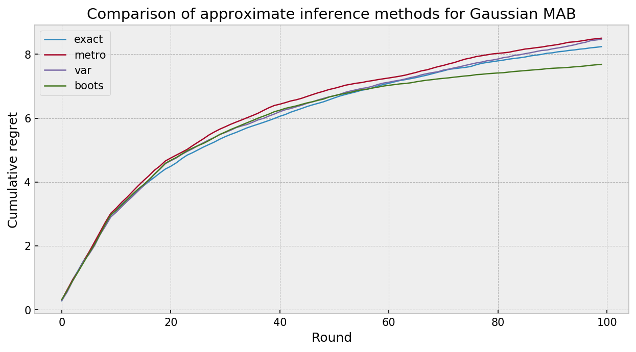
The plot below compares the cumulative regret for all of our inference algorithms paired with Thompson sampling, in 100 simulation of 10 rounds of gaussian bandit play. The approximate inference techniques fared very well, in what I would call a technical draw between methods. Variational Inference and MCMC were much slower than exact inference and bootstrapping. As the algorithms were given 10 observations at each round, bootstrapping did not suffer with lack of prior specification. Really cool results.
Conclusion
In this tutorial, we explored and compared approximate inference techniques to solve a gaussian bandit problem with Thompson Sampling. The central issue in approximate bayesian inference is to compute the posterior distribution $p(z\ \vert\ x) = \frac{p(x\ \vert\ z)\cdot{}p(z)}{p(x)}$. In general, in order to do that, we need to avoid computing the model evidence $p(x)$, which is most of the times intractable. MCMC Sampling techniques try to approximate the posterior with an empirical distribution built thorugh monte carlo samples taken according to the unnormalized posterior $p(x\ \vert\ z)\cdot{}p(z)$. Variational Inference, on the other hand, casts posterior inference as optimization, trying to find the variational distribution $q(z\ ;\ \lambda)$ that better approximates the posterior. It does that by minimizing the divergence between $q(z\ ;\ \lambda)$ and the unnormalized posterior $p(x\ \vert\ z)\cdot{}p(z)$, which works the same as minimizing divergence with respect to the true posterior. Bootstrapping approximates the posterior with an empirical distribution calculated by taking many bootstrap samples of the data. In our case, specifically, it was also possible to calculate the exact posterior to serve as a baseline for comparison.
Results were interesting. All approximate inference techniques did a good job approximating the exact posterior and showed similar performance in the gaussian bandit task. Bootstrapping was the most effcient, being faster than computing the exact posterior (as we only need to take one sample per action). VI and MCMC ran in similar time, as we need to only pass the burn-in to get the one sample per action for TS to work.
Given the results observed, Bootstrapping seems to be a good candidate as a approximate inference method for bandits, as it also accomodates very compex posteriors with virtually no model development cost. However, we should be aware of its lack of prior specification, which could negatively impact performance due to lack of exploration in early rounds.
What is your thought about this experiment? Feel free to comment! You can find the full code here.