Thompson Sampling is a very simple yet effective method to addressing the exploration-exploitation dilemma in reinforcement/online learning. In this series of posts, I’ll introduce some applications of Thompson Sampling in simple examples, trying to show some cool visuals along the way. All the code can be found on my GitHub page here.
In this post, we expand our Multi-Armed Bandit setting such that the expected rewards $\theta$ can depend on an external variable. This scenario is known as the Contextual bandit.
The Contextual Bandit
The Contextual Bandit is just like the Multi-Armed bandit problem but now the true expected reward parameter $\theta_k$ depends on external variables. Therefore, we add the notion of context or state to support our decision.
Thus, we’re going to suppose that the probabilty of reward now is of the form
\[\theta_k(x) = \frac{1}{1 + exp(-f(x))}\]where
\[f(x) = \beta_0 + \beta_1 \cdot x + \epsilon\]and $\epsilon \sim \mathcal{N}(0, \sigma^2)$. In other words, the expected reward parameters for each bandit linearly depends of an external variable $x$ with logistic link. Let us implement this in Python:
# class to implement our contextual bandit setting
class ContextualMAB:

    # initialization
    def __init__(self):

        # we build two bandits
        self.weights = {}
        self.weights[0] = [0.0, 1.6]
        self.weights[1] = [0.0, 0.4]

    # method for acting on the bandits
    def draw(self, k, x):

        # probability dict
        prob_dict = {}

        # loop for each bandit
        for bandit in self.weights.keys():

            # linear function of external variable
            f_x = self.weights[bandit][0] + self.weights[bandit][1]*x

            # generate reward with probability given by the logistic
            probability = 1/(1 + np.exp(-f_x))

            # appending to dict
            prob_dict[bandit] = probability

        # give reward according to probability
        return np.random.choice([0,1], p=[1 - prob_dict[k], prob_dict[k]]), max(prob_dict.values()) - prob_dict[k], prob_dict[k]
Let us visualize how the contexual MAB setting will work. First, let us see how the bandit probabilities depend on $x$. We set $\beta_0 = 0$ for both bandits, and $\beta_1 = 1.6$ for Bandit 0 and $\beta_1 = 0.4$ for Bandit 1.
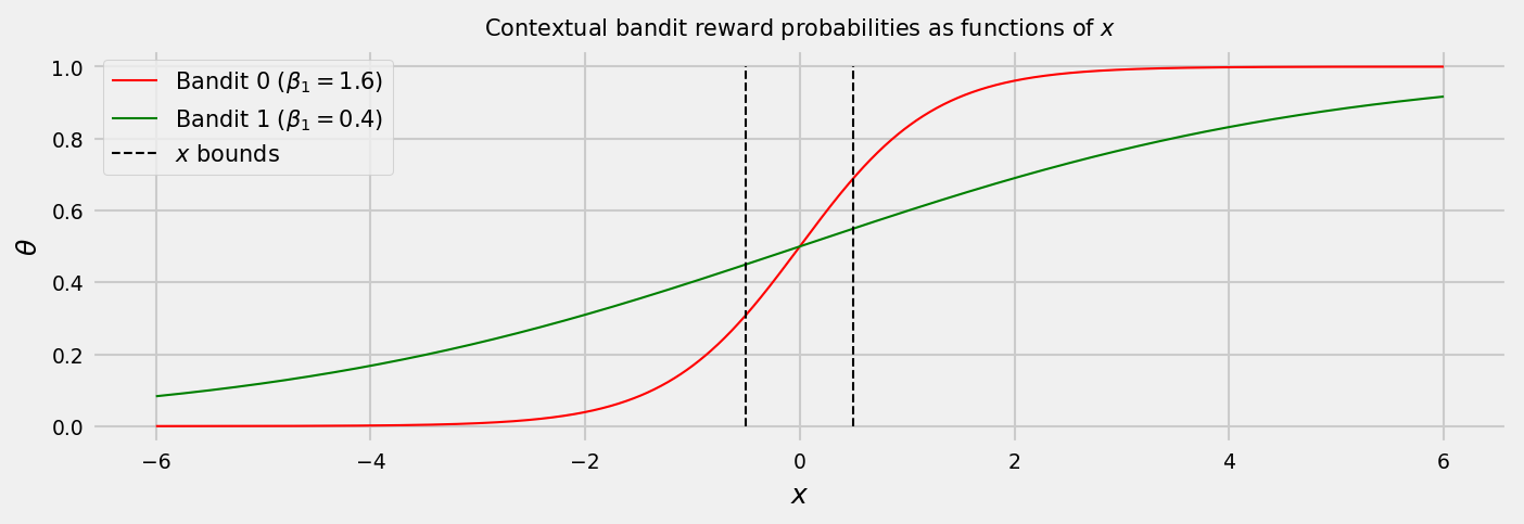
The plot shows us that an ideal strategy would select Bandit 0 if $x$ is greater than 0, and Bandit 1 if $x$ is less than 0. In the following plot, we show the bandits rewards over time depending on $x$ varying like a sine wave. The green and red shaded areas show the best action at each round.
We can see that more rewards pop up for Bandit 0 when $x$ is positive. Conversely, when $x$ is negative, Bandit 1 gives more rewards than Bandit 0. Let us implement an $\epsilon$-greedy policy and Thompson Sampling to solve this problem and compare their results.
Algorithm 1: $\epsilon$-greedy with regular Logistic Regression
Let us implement a regular logistic regression, and use an $\epsilon$-greedy policy to choose which bandit to activate. We try to learn the expected reward function for each bandit:
\[\theta_k(x) = \frac{1}{1 + exp(-f(x))}\]where
\[f(x) = \beta_0 + \beta_1 \cdot x + \epsilon\]And select the bandit which maximizes $\theta(x)$, except when, with $\epsilon$ probability, we select a random action (excluding the greedy action, which in our case is to draw the other arm).
The code for this is not very complicated:
# Logistic Regression with e-greedy policy class
class EGreedyLR:

    # initialization
    def __init__(self, epsilon, n_bandits, buffer_size=200):

        # storing epsilon, number of bandits, and buffer size
        self.epsilon = epsilon
        self.n_bandits = n_bandits
        self.buffer_size = buffer_size

    # function to fit and predict from a df
    def fit_predict(self, data, actual_x):

        # sgd object
        logreg = LogisticRegression(fit_intercept=False)

        # fitting to data
        logreg.fit(data['x'].values.reshape(-1,1), data['reward'])

        # returning probabilities
        return logreg.predict_proba(actual_x)[0][1]

    # decision function
    def choose_bandit(self, round_df, actual_x):

        # enforcing buffer size
        round_df = round_df.tail(self.buffer_size)

        # if we have enough data, calculate best bandit
        if round_df.groupby(['k','reward']).size().shape[0] == 4:

            # predictinng for two of our datasets
            bandit_scores = round_df.groupby('k').apply(self.fit_predict, actual_x=actual_x)

            # get best bandit
            best_bandit = int(bandit_scores.idxmax())

        # if we do not have, the best bandit will be random
        else:
            best_bandit = int(np.random.choice(list(range(self.n_bandits)),1)[0])

        # choose greedy or random action based on epsilon
        if np.random.random() > self.epsilon:
            return best_bandit
        else:
            return int(np.random.choice(np.delete(list(range(self.n_bandits)), best_bandit),1)[0])
Let us see a run of this algorithm. The green and red shaded areas show us which bandit should be played by an optimal strategy.
As we may see on multiple runs, it may take long for the e-greedy algorithm to start selecting the arms at the right times. It’s very likely that it gets stuck on a suboptimal actions for a long time.
Thompson Sampling may offer more efficient exploration. But how can we use it?
Algorithm 2: Online Logistic Regression by Chapelle et. al
In 2011, Chapelle & Li published the paper “An Empirical Evaluation of Thompson Sampling” that helped revive the interest on Thompson Sampling, showing favorable empirical results in comparison to other heuristics. We’re going to borrow the Online Logistic Regression algorithm (Algorithm 3) from the paper. Basically, it’s a bayesian logistic regression where we define a prior distribution for our weights $\beta_0$ and $\beta_1$, instead of just learning a point estimate for them (the expectation of the distribution).
So, our model, just like the greedy algorithm, is:
\[\theta_k(x) = \frac{1}{1 + exp(-f(x))}\]where
\[f(x) = \beta_0 + \beta_1 \cdot x + \epsilon\]but the weights are actually assumed to be distributed as independent gaussians:
\[\beta_i = \mathcal{N}(m_i,q_i^{-1})\]We initialize all $q_i$’s with a hyperparamenter $\lambda$, which is equivalent to the $\lambda$ used in L2 regularization. Then, at each new training example (or batch of examples) we make the following calculations:
- Find $\textbf{w}$ as the minimizer of $\frac{1}{2}\sum_{n=1}^{d} q_i(w_i - m_i)^2 + \sum_{j=1}^{n} \textrm{log}(1 + \textrm{exp}(1 + -y_jw^Tx_j))$
- Update $m_i = w_i$ and perform $q_i = q_i + \sum_{j=1}^{n} x_{ij}p_j(1-p_j)$ where $p_j = 1 + \textrm{exp}(1 + -w^Tx_j)^{-1}$ (Laplace approximation)
There are some heavy maths, but in essence, we basically altered the logistic regression fitting process to accomodate distributions for the weights. Our Normal priors on the weights are iteratively updated and as the number of observations grow, our uncertainty over them is reduced.
We can also increase incentives for exploration or exploitation by defining a hyperparameter $\alpha$, which multiplies the variance of the Normal posteriors at prediction time:
\[\beta_i = \mathcal{N}(m_i,\alpha \cdot{} q_i^{-1})\]With $0 < \alpha < 1$ we reduce the variance of the Normal priors, inducing the algorithm to be greedier, whereas with $\alpha > 1$ we prioritize exploration. Implementation of this algorithm by hand is a bit tricky. If you want to use a better code, with many possible improvements I would recommend skbayes. For now, let us use my craft OLR:
# defining a class for our online bayesian logistic regression
class OnlineLogisticRegression:

    # initializing
    def __init__(self, lambda_, alpha, n_dim):

        # the only hyperparameter is the deviation on the prior (L2 regularizer)
        self.lambda_ = lambda_; self.alpha = alpha

        # initializing parameters of the model
        self.n_dim = n_dim,
        self.m = np.zeros(self.n_dim)
        self.q = np.ones(self.n_dim) * self.lambda_

        # initializing weights
        self.w = np.random.normal(self.m, self.alpha * (self.q)**(-1.0), size = self.n_dim)

    # the loss function
    def loss(self, w, *args):
        X, y = args
        return 0.5 * (self.q * (w - self.m)).dot(w - self.m) + np.sum([np.log(1 + np.exp(-y[j] * w.dot(X[j]))) for j in range(y.shape[0])])

    # the gradient
    def grad(self, w, *args):
        X, y = args
        return self.q * (w - self.m) + (-1) * np.array([y[j] *  X[j] / (1. + np.exp(y[j] * w.dot(X[j]))) for j in range(y.shape[0])]).sum(axis=0)

    # method for sampling weights
    def get_weights(self):
        return np.random.normal(self.m, self.alpha * (self.q)**(-1.0), size = self.n_dim)

    # fitting method
    def fit(self, X, y):

        # step 1, find w
        self.w = minimize(self.loss, self.w, args=(X, y), jac=self.grad, method="L-BFGS-B", options={'maxiter': 20, 'disp':True}).x
        self.m = self.w

        # step 2, update q
        P = (1 + np.exp(1 - X.dot(self.m))) ** (-1)
        self.q = self.q + (P*(1-P)).dot(X ** 2)

    # probability output method, using weights sample
    def predict_proba(self, X, mode='sample'):

        # adding intercept to X
        #X = add_constant(X)

        # sampling weights after update
        self.w = self.get_weights()

        # using weight depending on mode
        if mode == 'sample':
            w = self.w # weights are samples of posteriors
        elif mode == 'expected':
            w = self.m # weights are expected values of posteriors
        else:
            raise Exception('mode not recognized!')

        # calculating probabilities
        proba = 1 / (1 + np.exp(-1 * X.dot(w)))
        return np.array([1-proba , proba]).T
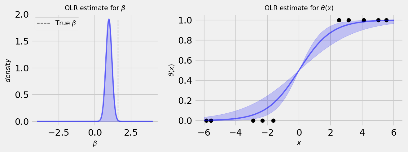
The following plot shows the Online Logistic Regression estimate for a simple linear model. The plot at the left-hand side shows the Normal posterior of the coefficient after fitting the model to some data. At the right-hand side, we can observe how the uncertainty in our coefficient translates to uncertainty in the prediction.
This way, it is very simple to use Thompson Sampling: we perform an OLR for each bandit, take a sample of the posterior of $\beta$, get the sampled output and choose the bandit with the highest prediction! Let us check one simulation:
TS shows a learning curve, but rapidly converges to the right decisions. We can control the amount of exploration using $\alpha$, with the trade-off of possibly being stuck on a suboptiomal strategy or to incur heavy costs for better exploring the set of actions at our disposal. You can fork the code at my GitHub and run the simulation many times with the parameters of your choosing.
When I first learned this algorithm, one thing that made me very curious is how the posterior distributions of the weights change over time. Let us take a look!
Visualizing the learning process
Let us visualize how the learning progresses and the model represents uncertainty. The following plot shows another episode using TS as the policy, along with the posterior distributions for $\beta_1$ for each bandit.
We see that in the first rounds our output probabilities have very large uncertainty and no clear direction. Also, our priors have large intersections, as the model is not very certain about its weights. As the rounds pass, we see that we effectively learn distributions for the weights and reduce our uncertainty around the output probabilities. When the model has low uncertainty, we start exploiting the bandits, choosing the best in each context.
Regret analysis
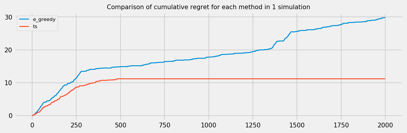
Finally, as in the last post, let us analyze the regret of the two policies with a longer simulation. We now draw the context from an uniform distribution. As simulations are expensive, particularly for TS (due to the Online Logistic Regression), we run only one simulation. We also add buffers to the algorithms, so they can remember only the most recent draws. The regret plot for both policies follows:
Conclusion
In this tutorial, we introduced the Contextual Bandit problem and presented two algorithms to solve it. The first, $\epsilon$-greedy, uses a regular logistic regression to get greedy estimates about the expeceted rewards $\theta(x)$. The second, Thompson Sampling, relies on the Online Logistic Regression to learn an independent normal distribution for each of the linear model weights $\beta_i \sim \mathcal{N}(m_i, q_i ^ -1)$. We draw samples from these Normal posteriors in order to achieve randomization for our bandit choices.
In this case, although Thompson Sampling presented better results, more experiments may be needed to declare a clear winner. The number of hyperparameters for both methods are the same: the regularization parameter $\lambda$ and the buffer size for both methods, $\epsilon$ for the $\epsilon$-greedy strategy and $\alpha$ for Thompson Sampling. Thompson Sampling may achieve the best results, but, in my experiments, it sometimes diverged depending on the hyperparameter configuration, completely inverting the correct bandit selection. The toy problem presented in this Notebook is very simple and may be not representative of the wild as well, so we may be better trusting the results on the Chapelle et. al paper. Last but not least, the time for fitting the Online Logistic Regression is an order of magnitude larger than fitting a regular logistic regression, which can still be improved if we use a technique like Stochastic Gradient Descent. In a big data context, it may be better to use a $\epsilon$-greedy stratedy for a while, then changing it to full exploitation at a some point given business knowledge. An $\epsilon$-decreasing strategy may be a good option as well.