
This is Zeca.
He’s bringing joy to our household for over a year now. He lives a happy life, with daily walks, good food, good healthcare, and a loving and caring family (myself and Bruna). Zeca’s the classic companion dog: a loyal, happy friend, good with people and children, and loves to be spoiled.
But it was not always like this. Zeca had a rough life until he could reach us. He was found at a back road tens of kilometres away from our current location, by a NGO that helps stray dogs find a family. His health was severely compromised, with malnutrition, skin issues and ear infection. He was afraid of people, and got really uneasy (and sometimes aggressive) when approached by humans (including myself and Bruna), indicating a history of violence. It was a privilege to see Zeca transform from a mistreated, fearful and unsociable dog to the healthy, happy and sociable companion he is today.
Now that we’re past all that, we have the luxury to think about more “trivial” questions when it comes to Zeca. Particularly, there’s two missing pieces of information that sparks debates in my family:
- Zeca’s breed (or lack thereof). The NGO said that he’s mixed-breed, where one of the elements of the mix is a poodle. Nevertheless, there’s a lot of uncertainty around that (he’s much bigger than a poodle, for instance).
- Zeca’s age. Estimates range from 2 years to 6 years, depending on source (NGO, vet, etc).
So I figured, why not try to come up with a data-driven answer to these questions? In this post, we’ll solve the mystery of Zeca’s breed using the Stanford Dogs Dataset, deep learning, and explainability through prototypes. Repository with code here.
Custom utilities
I built some custom utilities to isolate some core functionalities of my code. I’ll explain them in the post, but if you want to dig deeper please refer to this script on the repository.
# importing core
from dog_breeds_core import (build_metadata,
                             extract_features,
                             plot_embedding,
                             plot_dog_atlas,
                             get_prototypes_report)
Data
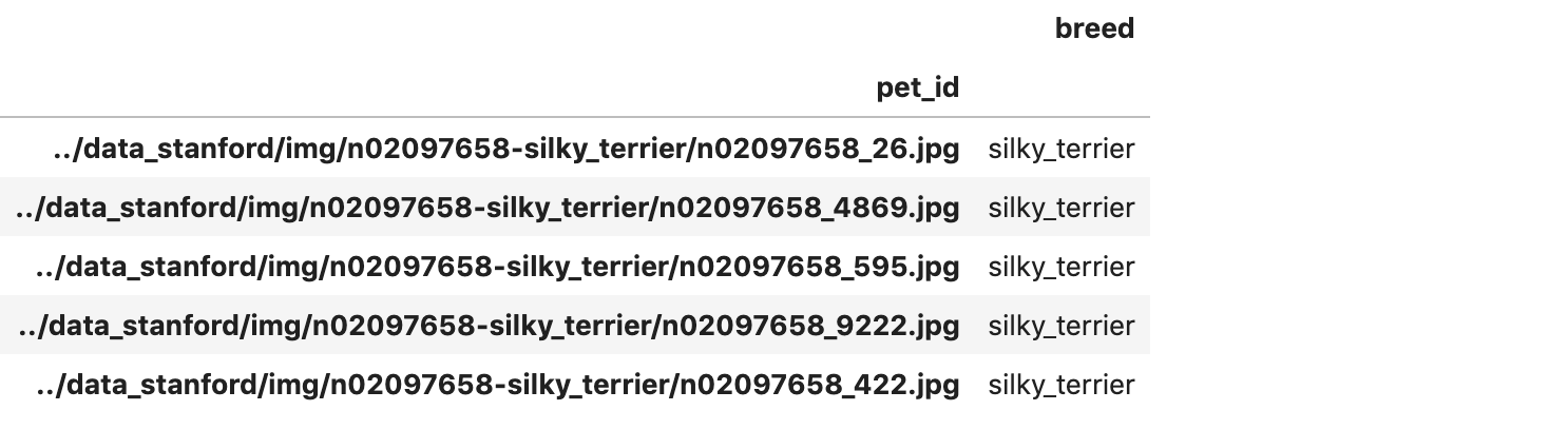
The data is divided into 120 folders, each representing a breed, that contain several dog pictures each. The build_metadata function builds a simple dataframe which contains a single column breed and the path to the corresponding image as index.
# reading data
meta_df = build_metadata()
meta_df.head()
As expected, we have 120 breeds. Also, we have 20580 images, as a I joined the train and test sets of the original dataset, as I need the most data I can get.
# number of unique breeds after filter
print('number of unique breeds:', meta_df['breed'].nunique())
print('number of rows in the dataframe:', meta_df['breed'].shape[0])
number of unique breeds: 120
number of rows in the dataframe: 20580
We reserve the images’ paths for use later:
# creating list with paths
paths = meta_df.index.values
Feature extraction
The first step is extracting features from the images using a pretrained neural network. I chose Xception based on its good results on this Kaggle Kernel, and for it being relatively lightweight for quick inference.
# using a pre-trained net
from tensorflow.keras.applications.xception import Xception, preprocess_input
from tensorflow.keras.preprocessing import image

# instance of feature extractor
extractor = Xception(include_top=False, pooling='avg')
The function extract_features gets a list of paths, an extractor (the Xception net in this case), and returns a dataframe with features. We save the dataframe so we don’t need to run the process all the time (it takes ~15 minutes on my machine).
# if we havent extracted features, do it
if not os.path.exists('../data_stanford/features.csv'):
    features_df = extract_features(paths, extractor)
    features_df.to_csv('../data_stanford/features.csv')

# read features
features_df = pd.read_csv('../data_stanford/features.csv', index_col='pet_id')
As the extraction pipeline can’t process some of the images, we need to realign our metadata index with the extraction’s index, so they have the same images, in the same order:
# realign index with main df
meta_df = meta_df.loc[features_df.index]
Modeling
Now we can start modeling. We’ll build a Logistic Regression to classify breeds on top of the Xception’s features, and apply this model on a picture of Zeca. However, for the sake of explainability, we’ll also create a nearest-neighbors model, so we can supply prototypes, comparable dogs to Zeca that can support the model’s predictions.
Let’s start with data preparation!
Data preparation
Just explicitly splitting our design matrix X and target variable y into train and test sets (90%/10% split, stratified). We encode y using LabelEncoder as this is a multiclass classification problem.
# label encoder for target and splitter
from sklearn.preprocessing import LabelEncoder
from sklearn.model_selection import train_test_split

# defining design matrix
X = features_df.copy().values

# defining target
label_encoder = LabelEncoder()
y = label_encoder.fit_transform(meta_df['breed'])

# splitting train and test
X_train, X_test, y_train, y_test = train_test_split(X, y, test_size=0.1, stratify=y)
Dimensionality reduction with PCA
We run PCA in the Xception’s features. We have two reasons for that:
- Efficiency. PCA can retain 96% of variance with half the features (1024 instead of 2048). This helps everything run faster further in the pipeline.
- Whitening. Whitening is the PCA’s capability of returning a matrix where features have mean 0, variance 1, and are uncorrelated. This will be important as it allows us to interpret the Logistic Regression coefficients as feature importances.
We fit PCA with the following code:
# PCA
from sklearn.decomposition import PCA

# instance of PCA
pca = PCA(n_components=1024, whiten=True)

# applying PCA to data
# must only fit on train data
pca.fit(X_train)

# checking explained variance
explained_var = pca.explained_variance_ratio_.sum()
print(f'PCA explained variance: {explained_var:.4f}')
PCA explained variance: 0.9646
Logistic Regression
We then proceed to fit and evaluate a Logistic Regression. It’s fairly easy and fast to fit it:
# logistic regression and eval metrics
from sklearn.linear_model import LogisticRegression
from sklearn.metrics import accuracy_score, log_loss

# instance of logistic regression
lr = LogisticRegression(C=1e-2, multi_class='multinomial', penalty='l2', max_iter=200)

# fitting to train
lr.fit(pca.transform(X_train), y_train)
And it gives a pretty reasonable result: 88% accuracy on 120 breeds!
# evaluating
val_preds = lr.predict_proba(pca.transform(X_test))

# test metrics
print(f'Accuracy: {accuracy_score(y_test, np.argmax(val_preds, axis=1)):.3f}')
print(f'Log-loss: {log_loss(y_test, val_preds):.3f}')
Accuracy: 0.881
Log-loss: 0.523
Predicting breed for Zeca
For the moment we’ve been waiting for. What is Zeca’s breed? I’ll use the following image, as he’s on a better pose:

We just run feature extraction on the image and get the top breeds for Zeca:
# features from zeca
features_zeca = extract_features([f'../data_stanford/target_imgs/zeca.jpg'], extractor)

# predictions for zeca
preds_zeca = lr.predict_proba(pca.transform(features_zeca))[0]
preds_zeca = pd.Series(preds_zeca, index=label_encoder.classes_)
preds_zeca.sort_values(ascending=False).to_frame().head(10)
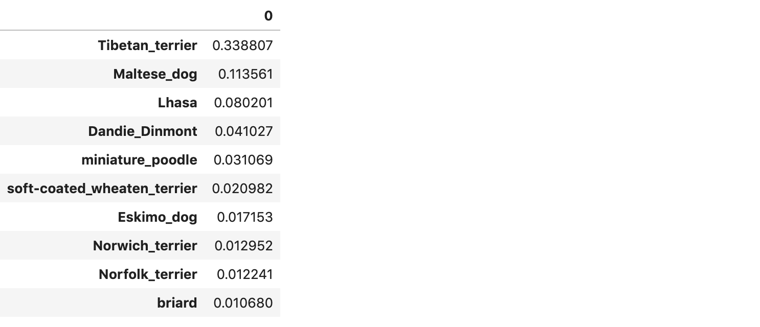
The top candidate is the Tibetan Terrier, followed by the Maltese, Lhasa and Dandie Dinmont. Cool! It makes a lot of sense to me. My uncle owns a Maltese, and I’ve once called Zeca a “giant Maltese”. Our first candidate, the Tibetan Terrier, shows a very close resemblance. Look at this dog that I’ve found searching for Tibetan Terrier on Google:

It’s very, very close. But we can’t call this a victory yet. One could also find this image on the same search:
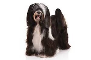
Which is not very close, and will warrant me a defeat when I present my conclusions to my family. How can we know that the model is making good decisions?
Explanations via embeddings and prototypes
One easy and effective method that I usually apply for explaining models is trying to transform them in a kNN (yeah, nearest neighbors!), as it outputs hard examples to support the model’s decisions (or prototypes, as in the literature). How do we transform our Xception + PCA + Logistic Regession pipeline in a kNN, though? I’ll show you two ways:
- Direct, naive way: Just search for Zeca’s neighbors in the
Xception+PCAfeature space - Scale by Logistic Regression coefficients: we apply a bit of supervision on the
Xception+PCAembedding, scaling its features proportionally to the weights of the Logistic Regression.
Let us check how they perform. We start by importing NNDescent, a fast, efficient method to perform approximate nearest neighbor search:
# nearest neighbors
from pynndescent import NNDescent
Direct, naive embedding
Now, we search for Zeca’s comparables in a naive way. It consists of creating an index on the Xception + PCA embedding, and then searching for zeca’s neighbors in this index. The function get_prototypes_report takes care of that for us, and shows pictures and most frequent breeds for Zeca’s neighbors:
# creating NN index
index_direct = NNDescent(pca.transform(X))

# running
get_prototypes_report(f'../data_stanford/target_imgs/zeca.jpg', index_direct, extractor, pca.transform, meta_df, features_df)
Most Frequent Breeds:
Lhasa                   0.20
Maltese_dog             0.16
Tibetan_terrier         0.12
EntleBucher             0.06
Bernese_mountain_dog    0.04
Blenheim_spaniel        0.04
malamute                0.04
Old_English_sheepdog    0.04
silky_terrier           0.02
Shetland_sheepdog       0.02
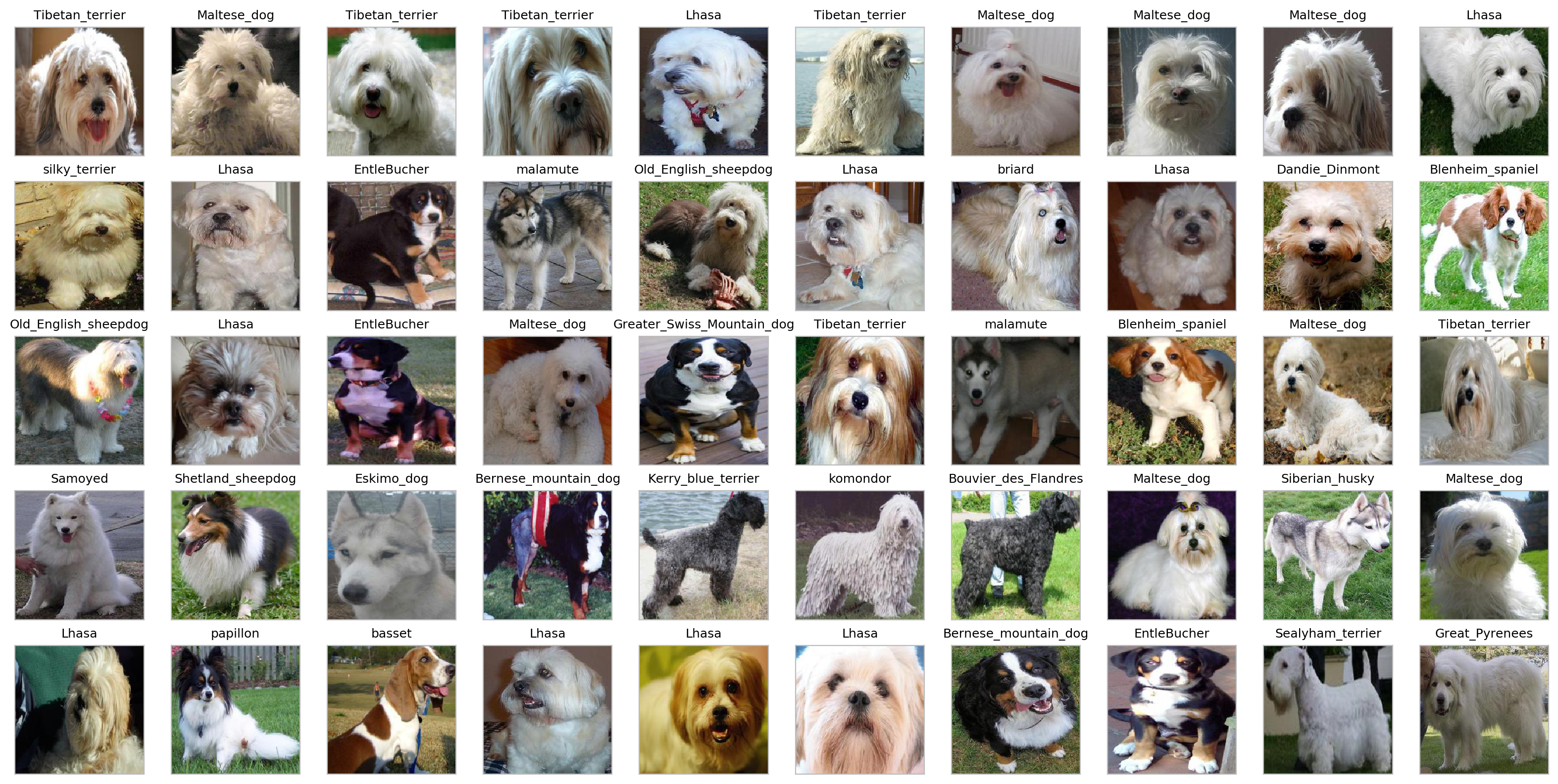
We start off OK on the first 10 dogs, but we get neighbors that don’t make much sense, like the EntleBucher or Bouvier_des_Flandres. Let us then improve that by applying a bit of supervision using the logistic regression’s weights.
Scale by Logistic Regression coefficients
Let us perform a very simple modification to the embedding that our nearest neighbor method builds its index on. We use the fact that we can interpret the absolute value of the coefficients of the Logistic Regression as feature importances (as allowed by the whitening process), and scale the embedding features proportionally to these coefficients.
For instance, we can check that there are some features with nearly 10x more importance than others:
# checking feature importance
np.abs(lr.coef_).sum(axis=0)
array([10.60028291,  9.96382911, 10.35478674, ...,  1.58498523,
        1.82601082,  1.93528317])
So, when we scale the embedding this way, the Logistic Regression’s most important features will have greater variance, and thus will have more weight when we search for Zeca’s nearest neighbors:
# function to 'supervise' embedding given coefficients of logreg
lr_coef_transform = lambda x: np.abs(lr.coef_).sum(axis=0) * pca.transform(x)

# creating NN index
index_logistic = NNDescent(lr_coef_transform(X))
The results are much better:
# running
get_prototypes_report(f'../data_stanford/target_imgs/zeca.jpg', index_logistic, extractor, lr_coef_transform, meta_df, features_df)
Most Frequent Breeds:
Lhasa                          0.32
Tibetan_terrier                0.24
Maltese_dog                    0.24
Dandie_Dinmont                 0.10
silky_terrier                  0.04
soft-coated_wheaten_terrier    0.02
briard                         0.02
miniature_poodle               0.02
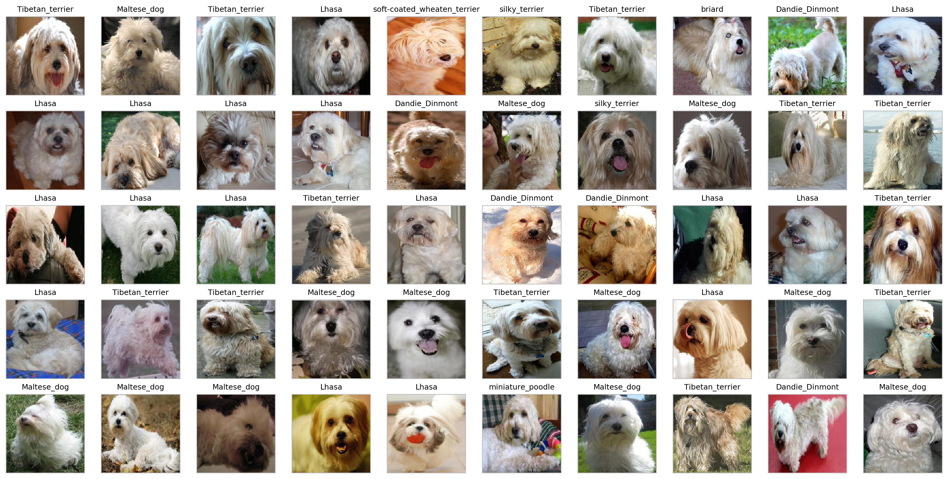
The prototypes agree a lot with the Logistic Regression results, and they’re gonna be a solid argument for my family that the model works.
Digging deeper: Why did the supervision work?
Why did simple scaling improve prototype quality by so much? My hypothesis is based on the curse of dimensionality. To check that, let us compare the 2D embedding generated by UMAP from the naive and scaled approaches.
We generate the embeddings with the following code:
# UMAP for dimension reduction
from umap import UMAP

# building embedding
umap_direct = UMAP()
embed_direct = umap_direct.fit_transform(pca.transform(X))

# predicting zeca
zeca_embed_direct = umap_direct.transform(pca.transform(features_zeca))

# building embedding
umap_logistic = UMAP()
embed_logistic = umap_logistic.fit_transform(lr_coef_transform(X))

# predicting zeca
zeca_embed_logistic = umap_logistic.transform(lr_coef_transform(features_zeca))
And plot them below:
# opening figure
plt.figure(figsize=(16, 6), dpi=150)

# plotting 2D reduction of naive embedding
plt.subplot(1, 2, 1)
plot_embedding(embed_direct, zeca_embed_direct, 'Color is Breed: embedding directly from network', y)

# plotting 2D reduction of scaled embedding
plt.subplot(1, 2, 2)
plot_embedding(embed_logistic, zeca_embed_logistic, 'Color is Breed: embedding scaled by logistic regression weights', y)
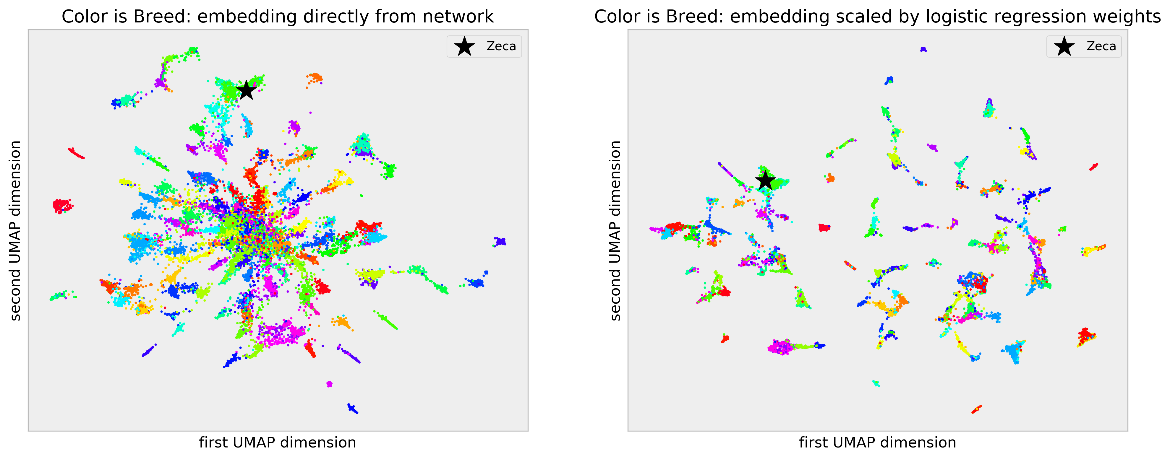
Breed is color-coded in the plots. The naive embedding plot, in the left-hand side, shows reasonable structure, with some clear clusters of breeds clumping together. However, there’s a “hubness” problem: there’s a central clump of dog images where there’s a lot of mix between breeds. I make my case that this is the curse of dimensionality at play: the 1024 features we get from the Xception and PCA are suited to a much more general problem of object idenfitication and are “too sparse” for our dog breed classification problem. Thus, we end up comparing pictures on features that don’t make sense for our specific problem, making dogs that are different appear the same (and the contrary as well).
In the right-hand plot, built from the scaled embedding, we get much tighter, cleaner clusters, with no “hubness” at all. The scaling process acts like a “filter” letting we only compare pictures of dogs on the features that are important for our specific task of dog breed identification, as determined by our model. It’s like learning a distance between our entities given our task.
For your amusement, I can also generate these plots using dog pictures. Here’s what I call the Dog Atlas:
# opening figure
fig, ax = plt.subplots(1, 2, figsize=(16, 6), dpi=150)

# plotting atlas
plot_dog_atlas(embed_direct, meta_df, 'Dog Atlas: naive embedding', ax[0])
plot_dog_atlas(embed_logistic, meta_df, 'Dog Atlas: scaled embedding', ax[1])
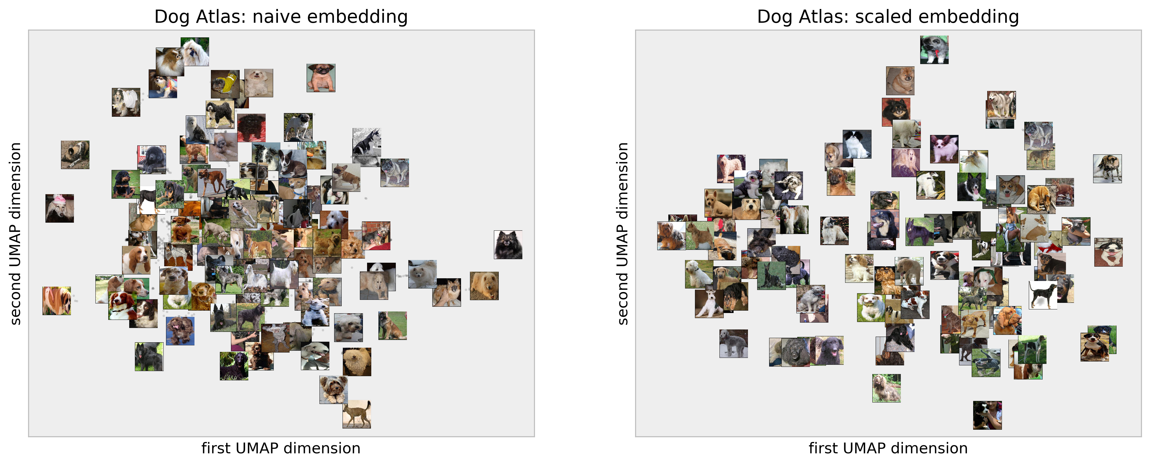
Cool! It’s a fluffier way to see that the scaled embedding is better :)
Final Remarks
Cool! We solved the mistery of Zeca’s breed. We did not solve age, though, as we did not have the labels. I’ll try on a next project.
Thank you very much for reading! Comments and feedbacks are appreciated :)