One of the biggest issues in causal inference problems is confounding, which stands for the impact explanatory variables may have on treatment assignment and the target. To draw conclusions on the causality of a treatment, we must isolate its effect, controlling the effects of other variables. In a perfect world, we would observe the effect of a treatment in identical individuals, inferring the treatment effect as the difference in their outcomes.

Sounds like an impossible task. However, ML can help us in it, providing us with individuals that are “identical enough”. A simple and effective way to do this is using a decision tree. I’ve shown before that decision trees can be good causal inference models with some small adaptations, and tried to make this knowledge acessible through the cfml_tools package. They are not the best model out there, however, they show good results, are interpretable, simple, and fast.

The methodology is as follows: we build a decision tree to solve a regression or classification problem from explanatory variables X to target y, and then compare outcomes for every treatment W at each leaf node to build counterfactual predictions. Recursive partitioning performed by the tree will create clusters with individuals that are “identical enough” and enable us to perform counterfactual predictions.

But that is not always true. Not all partitions are born equal, and thus we need some support to diagnose where inference is valid and where it may be biased. In this Notebook, we’ll use the .run_leaf_diagnostics() method from DecisionTreeCounterfactual which helps us diagnose that, and check if our counterfactual estimates are reasonable and unconfounded.

Data: make_confounded_data from fklearn

Nubank’s fklearn module provides a nice causal inference problem generator, so we’re going to use the same data generating process and example from its documentation.

from cfml_tools.utils import make_confounded_data
df_rnd, df_obs, df_cf = make_confounded_data(500000)
print(df_to_markdown(df_obs.head(5)))

sex	age	severity	medication	recovery
0	35	0.85	1	19
1	38	0.52	1	32
1	42	0.7	1	24
1	25	0.54	1	19
0	16	0.34	0	17

We have five features: sex, age, severity, medication and recovery. We want to estimate the impact of medication on recovery. So, our target variable is recovery, our treatment variable is medication and the rest are our explanatory variables. Additionally, the function outputs three data frames: df_rnd, where treatment assingment is random, df_obs, where treatment assingment is confounded and df_cf, which is the counterfactual dataframe, with the treatment indicator flipped.

The real effect is $\frac{E[y \mid W=1]}{E[y \mid W=0]} = exp(-1) = 0.368$. We use df_obs to show the effects of confounding.

Decision Trees as causal inference models

Let us do a quick refresher on the usage of the DecisionTreeCounterfactual method. First, we organize data in X, W and y format:

# organizing data into X, W and y
X = df_obs[['sex','age','severity']]
W = df_obs['medication'].astype(int)
y = df_obs['recovery']

Then, we fit the counterfactual model. The default setting is a minimum of 100 samples per leaf, which (in my experience) would be reasonable for most cases.

# importing cfml-tools
from cfml_tools.tree import DecisionTreeCounterfactual

# instance of DecisionTreeCounterfactual
dtcf = DecisionTreeCounterfactual(save_explanatory=True)

# fitting data to our model
dtcf.fit(X, W, y)

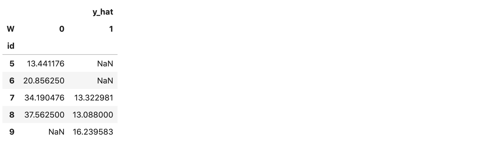
We then predict the counterfactuals for all our individuals. We get the dataframe in the counterfactuals variable, which predicts outcomes for both W = 0 and W = 1.

We can see some NaNs in the dataframe. That’s because for some individuals there are not enough treated or untreated samples at the leaf node to estimate the counterfactuals, controlled by the parameter min_sample_effect. When this parameter is high, we are conservative, getting more NaNs but less variance in counterfactual estimation.

# let us predict counterfactuals for these guys
counterfactuals = dtcf.predict(X)
counterfactuals.iloc[5:10]

We check if the underlying regression from Xto y generalizes well, with reasonable R2 scores:

# validating model using 5-fold CV
cv_scores = dtcf.get_cross_val_scores(X, y)
print(cv_scores)

[0.60043037 0.60253992 0.59829968 0.60939054 0.60682531]

We want to keep this as high as possible, so we can trust that the model “strips away” the effects from X to y.

Then we can observe the inferred treatment effect, which the model retrieves nicely:

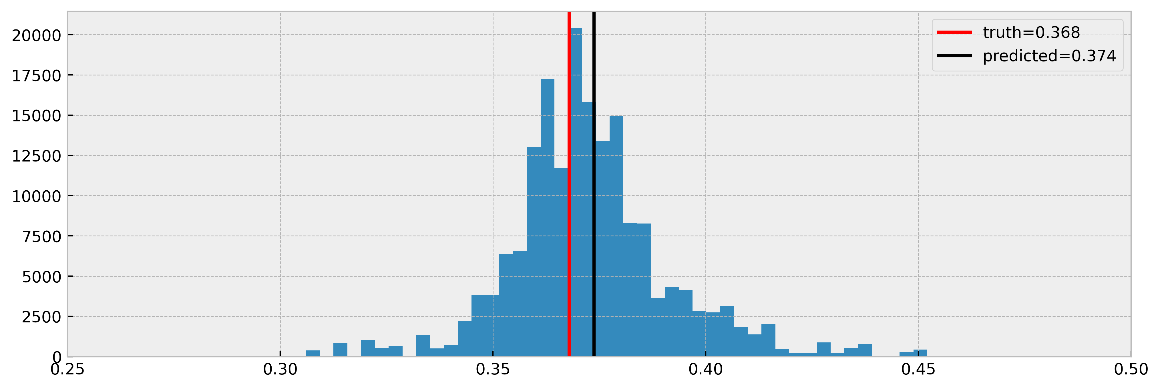
However, it is not perfect. We can observe that some estimates are way over the real values. Also, in a real causal inference setting the true effect would not be acessible as an observed quantity. That’s why we perform CV only to diagnose the model’s generalization power from Xto y. For the treatment effect, we have to trust theory and have a set of diagnostic tools at our disposal. That’s why we built .run_leaf_diagnostics() :). We’ll show it in the next section.

Digging deeper with leaf diagnostics

The .run_leaf_diagnostics() method provides valuable information to diagnose the countefactual predictions of the model. It performs analysis over the leaf nodes, testing if they really are the clusters containing the “identical enough” individuals we need.

We run the method and get the following dataframe:

# running leaf diagnostics
leaf_diagnostics_df = dtcf.run_leaf_diagnostics()
leaf_diagnostics_df.head()

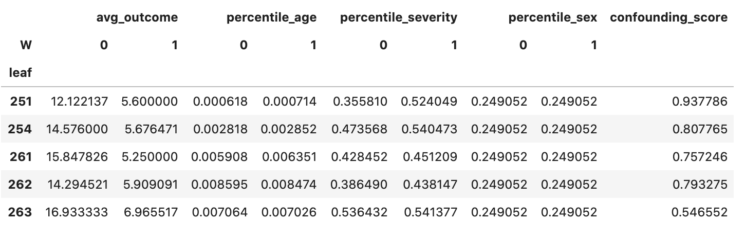
The dataframe provides a diagnostic on leaves with enough samples for counterfactual inference, showing some interesting quantities:

• average outcomes across treatments (avg_outcome)
• explanatory variable distribution across treatments (percentile_* variables)
• a confounding score for each variable, meaning how much we can predict the treatment from explanatory variables inside leaf nodes using a linear model (confounding_score)

The most important column is the confounding_score, which tells us if treatments are not randomly assigned within leaves given explanatory variables. It is actually the AUC of a linear model that tries to tell treated from untreated individuals apart within each leaf. Let us check how our model fares on this score:

# avg confounding score
confounding_score_mean = leaf_diagnostics_df['confounding_score'].median()

# plotting
plt.figure(figsize=(12,6), dpi=120)
plt.axvline(
    confounding_score_mean,
    linestyle='dashed',
    color='black',
    label=f'Median confounding score: {confounding_score_mean:.3f}'
)
plt.hist(leaf_diagnostics_df['confounding_score'], bins=100)
plt.legend()

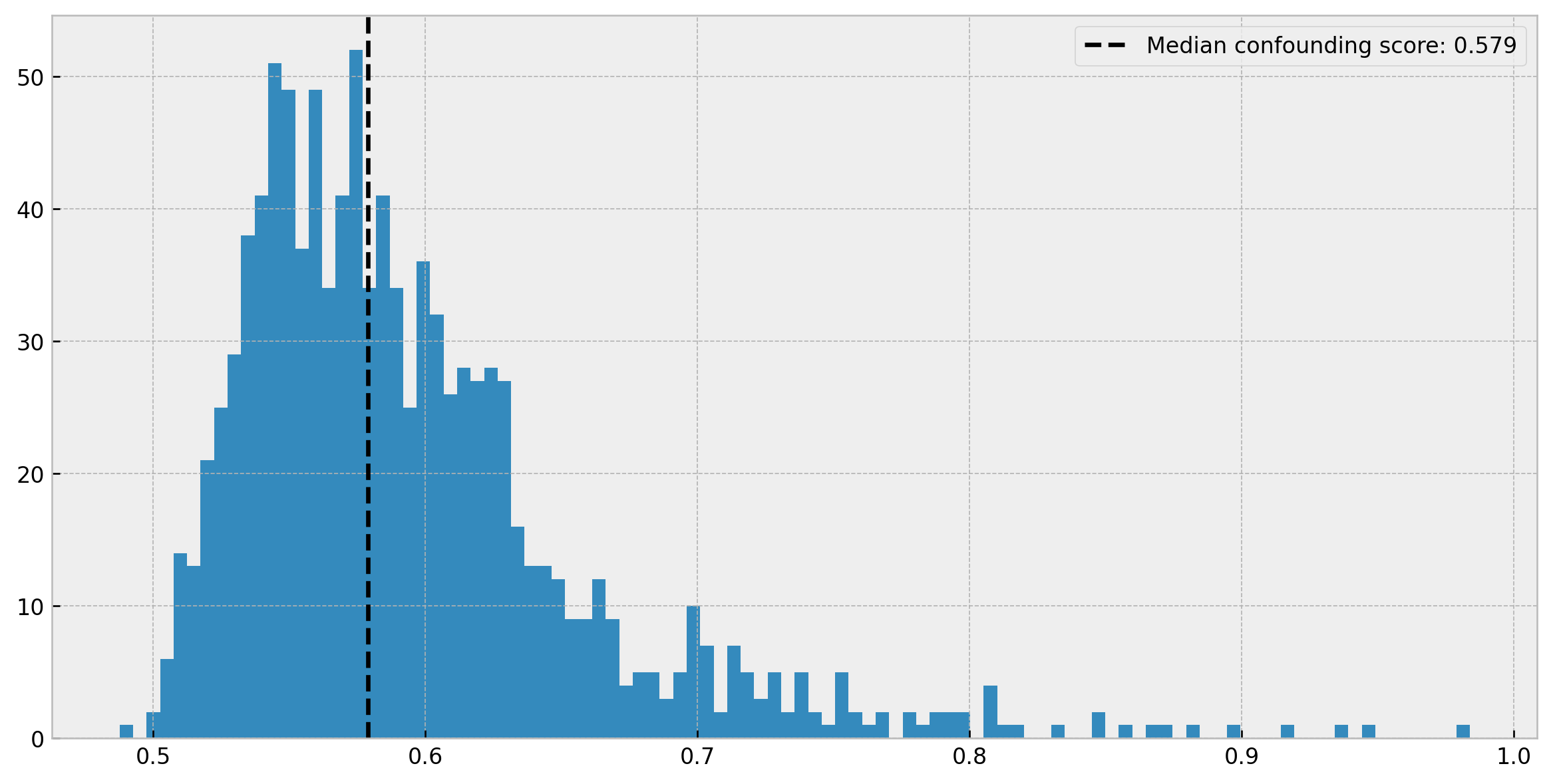
Cool. This is a good result, as within more than half of the leaves treated and untreated individuals are virtually indistinguishable (AUC less than 0.6). However, we can check that for some of the leaves we have a high confounding score. Therefore, in those cases, our individuals may not be “identical enough” and inference may be biased.

We actually can measure how biased inference can be. Let us plot how the confounding score impacts the estimated effect.

# adding effect to df
leaf_diagnostics_df = (
    leaf_diagnostics_df
    .assign(effect=lambda x: x['avg_outcome'][1]/x['avg_outcome'][0])
)

# real effect of fklearn's toy problem
real_effect = np.exp(-1)

# plotting
fig, ax = plt.subplots(1, 1, figsize=(12,6), dpi=120)

plt.axhline(
    real_effect,
    linestyle='dashed',
    color='black',
    label='True effect'
)

leaf_diagnostics_df.plot(
    x='confounding_score',
    y='effect',
    kind='scatter',
    color='tomato',
    s=10,
    alpha=0.5,
    ax=ax
)

plt.legend()

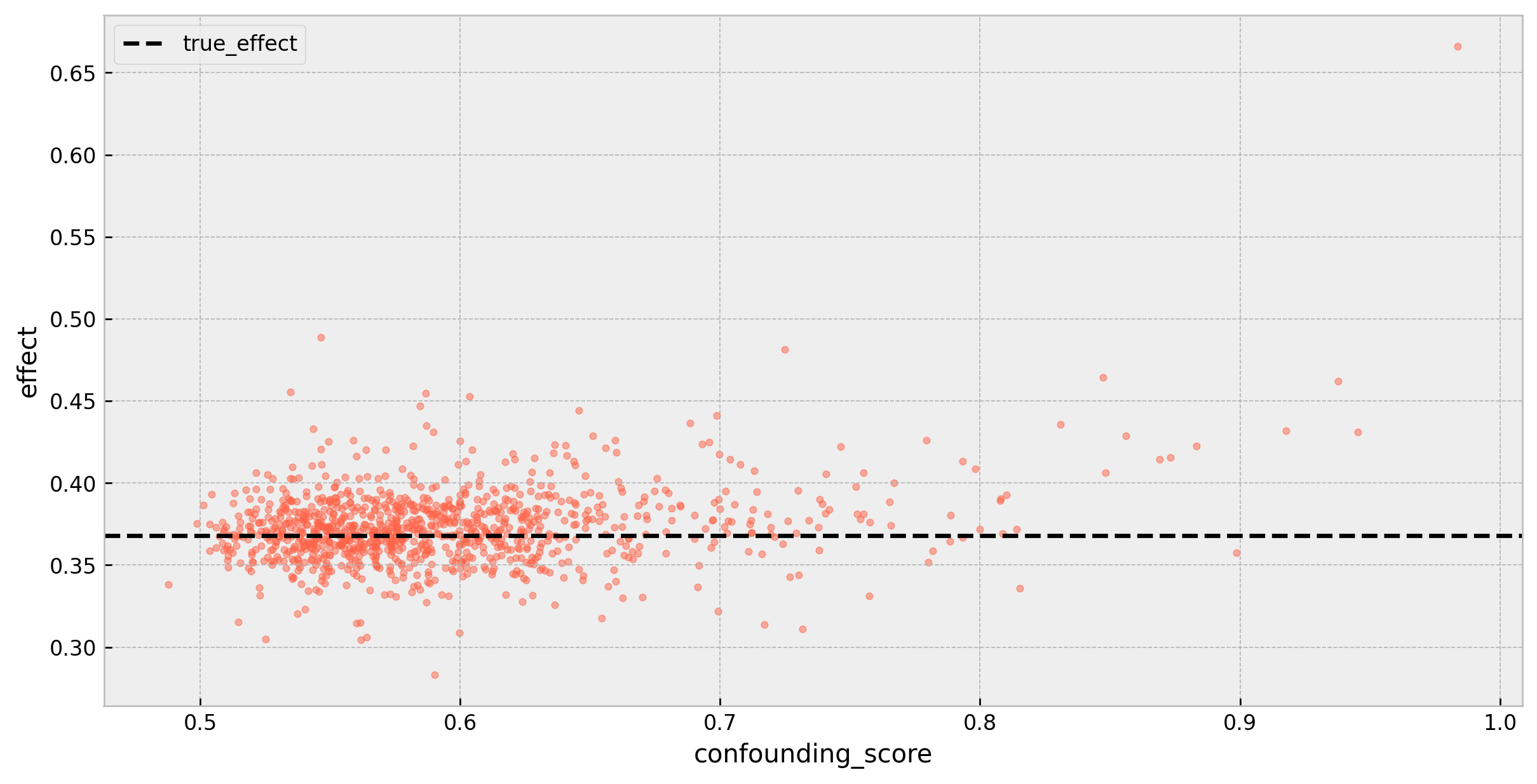
As we can see, there’s a slight bias that presents itself with higher confounding scores:

effect_low_confounding = (
    leaf_diagnostics_df
    .loc[lambda x: x.confounding_score < 0.6]
    ['effect'].mean()
)

effect_high_confounding = (
    leaf_diagnostics_df
    .loc[lambda x: x.confounding_score > 0.8]
    ['effect'].mean()
)

print(f'Effect for leaves with confounding score < 0.6: {effect_low_confounding:.3f}')
print(f'Effect for leaves with confounding score > 0.8: {effect_high_confounding:.3f}')

Effect for leaves with confounding score < 0.6: 0.371
Effect for leaves with confounding score > 0.8: 0.421

Let’s examine the leaf with the highest confounding score:

# leaf with highest confounding score
leaf_diagnostics_df.sort_values('effect', ascending=False).head(1)

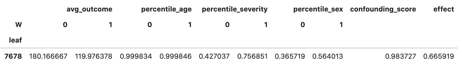
It shows a confounding score of 0.983, so we can almost perfectly tell treated and untreated individuals apart using the explanatory variables. The effect is grossly underestimated, as $log(0.665) = -0.408$. Checking the feature percentiles, we can see a big difference in severity and sex for treated and untreated individuals.

We can check these differences further by leveraging the stored training dataframe and building a boxplot:

# getting the individuals from biased leaf
biased_leaf_samples = dtcf.train_df.loc[lambda x: x.leaf == 7678]

# plotting
fig, ax = plt.subplots(1, 4, figsize=(16, 5), dpi=150)
biased_leaf_samples.boxplot('age','W', ax=ax[0])
biased_leaf_samples.boxplot('sex','W', ax=ax[1])
biased_leaf_samples.boxplot('severity','W', ax=ax[2])
biased_leaf_samples.boxplot('y','W', ax=ax[3])

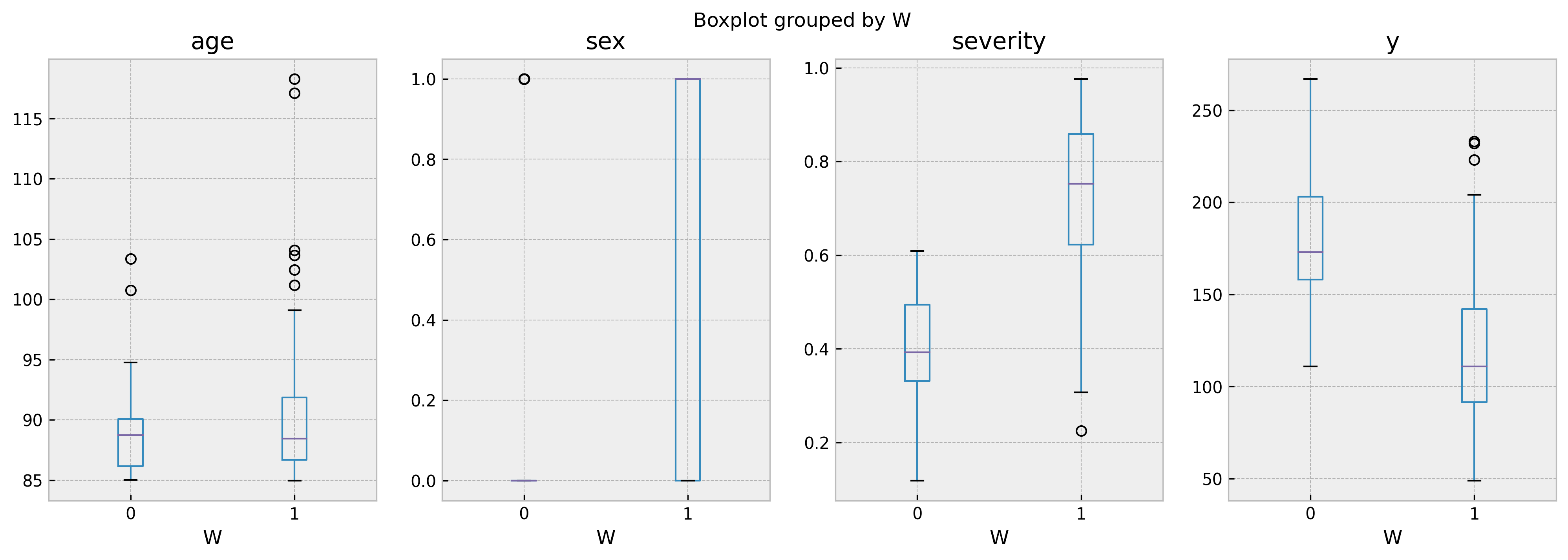
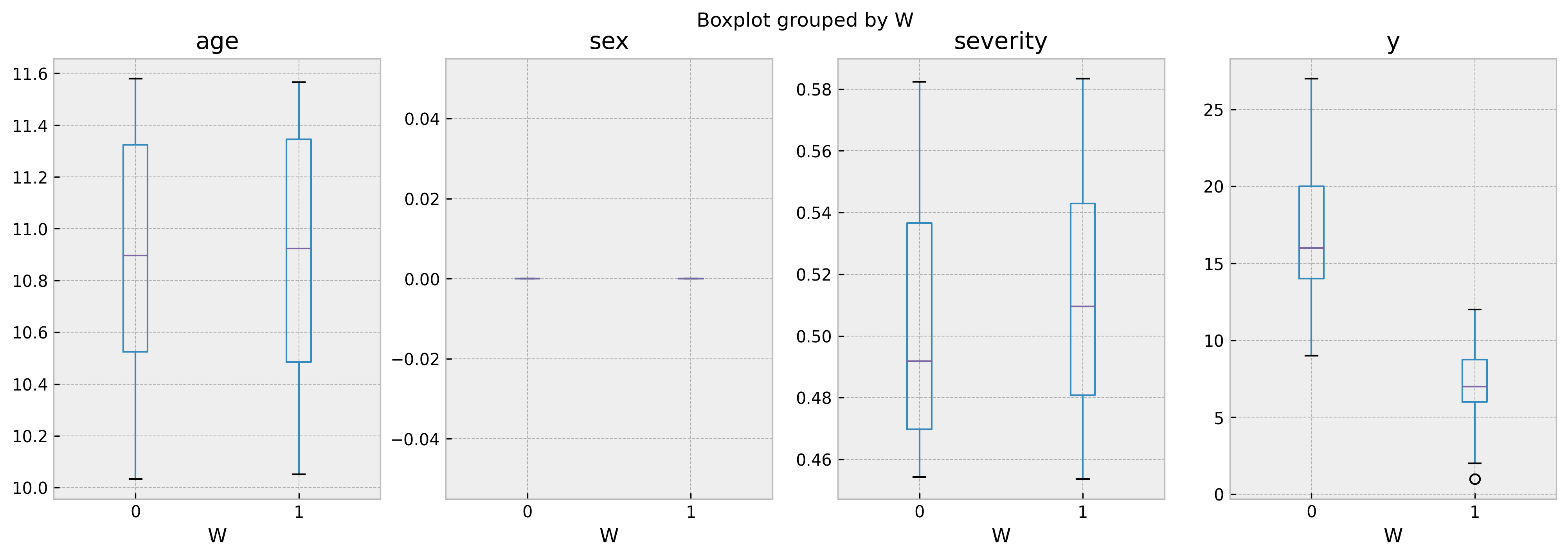
As we can see, ages are comparable but sex and severity are not. In a unbiased leaf, such as 263 (with confounding score of 0.54), the boxplots show much more homogenous populations:

# getting the individuals from biased leaf
biased_leaf_samples = dtcf.train_df.loc[lambda x: x.leaf == 263]

# plotting
fig, ax = plt.subplots(1, 4, figsize=(16, 5), dpi=150)
biased_leaf_samples.boxplot('age','W', ax=ax[0])
biased_leaf_samples.boxplot('sex','W', ax=ax[1])
biased_leaf_samples.boxplot('severity','W', ax=ax[2])
biased_leaf_samples.boxplot('y','W', ax=ax[3])

And that’s it! I hope this post help you in your journey to accurate, unbiased counterfactual predictions. All feedbacks are appreciated!